
Psy 232 Stats/Methods II
Analyzing Ordinal Data
I. Mann-Whitney Test
Used with ordinal data from two separate samples to evaluate the difference between two treatment conditions or populations.
An alternative to the independent-measures t-test
Ordinal data = rank-ordered data
Remember how we assigned ranks for the Spearman
rank-order correlation coefficient?
Use the same process here.
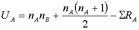
General idea: If a real difference between the two treatments exists, the scores in one sample should be generally larger than the scores in the second sample. When all scores are rank-ordered, the scores from one sample should be concentrated on one end and the scores from the other sample should be concentrated on the other end.
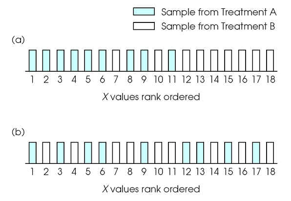
To determine whether the two samples are systematically clustered at opposite ends of the scale we must compute U.
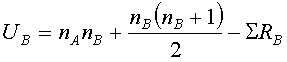
U computes points for each of the two samples (UA and UB)as if they were competing against each other.
The final Mann-Whitney U is the smaller of these two values.
Can count points manually or use the following formulas:
Ho states that there is no real difference between the two populations from which the samples are selected.
If Ho is true, then the U value will be relatively large
If Ho is false, then the U value will be near zero
Look up the critical value of U from Table B.9 (P. 712 for alpha = .05 and p. 713 for alpha = .01).
For future reference:
When both samples are n = 20 or higher, then the Mann-Whitney U
distribution will be approximately normal in shape. Therefore, we use the normal
approximation with larger samples.
Find the U values for each sample (as above). When the final U has been determined, perform the following calculations to locate U in the normal distribution.

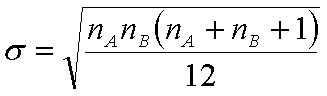
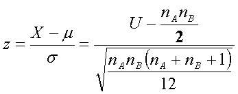
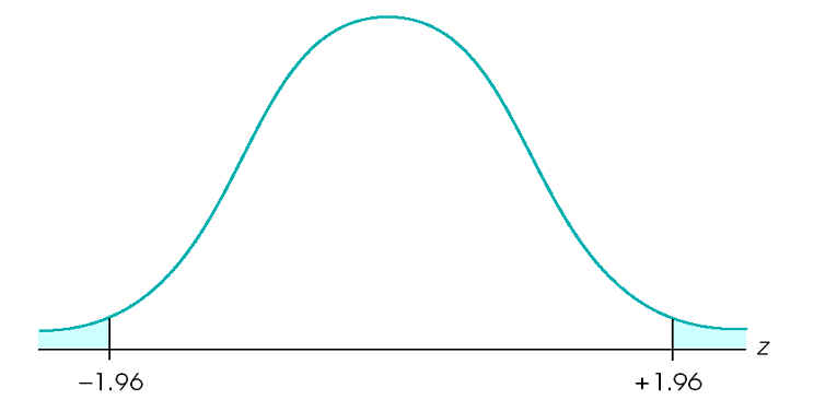
Use the unit normal table to define the critical region for the calculated z-score.
II. Wilcoxon Signed-Ranks Test
Used with ordinal data from a repeated-measures design to evaluate the difference between two treatments.
Analogous to a paired-samples (repeated-measures) t-test.
The Wilcoxon test focuses on the difference score for each individual.
Difference scores must be ranked from smallest to largest in terms of their absolute values. Then compute the sums of the ranks for (1) the positive difference scores and (2) the negative difference scores.
The smaller of these two sums becomes the final test statistic called the Wilcoxon T.
If a treatment effect exists
A strong treatment effect should cause the difference scores to be
consistently positive or consistently negative. If all of the differences are in
the same direction, the Wilcoxon T will be 0.
If a treatment effect does NOT exist
The signs of the difference scores should be intermixed evenly between
negative and positive. The Wilcoxon T will then be relatively large.
Look up the critical value of T in Table B.10 on page 714.
Continuity Assumption: The dependent variable is continuous, making duplicate scores very unlikely. Like the Mann-Whitney test, the Wilcoxon test is only appropriate when there are "relatively few" ties.
Dealing with tied scores and difference scores of 0
Tied scores occur when two or more participants have identical difference scores (ignoring the sign).
As we've dealt with ranks before, assign the average of the tied ranks.
Difference scores of 0 occur when a participant's score is the same in both treatment 1 and treatment 2.
Can discard these individuals from the analysis and adjust n accordingly. (NOT the preferred method, Why?)
Can divide the zero difference scores evenly between the positive and negative groups. If an odd number, discard one so the remaining zero scores can be divided evenly. (Preferred)
III. Kruskal-Wallis Test
Used with ordinal data from a between-subjects design with three or more treatment conditions (groups)
The groups can represent different treatment conditions or different levels of a subject variable (e.g., gender or age)
The Ho states that there is no tendency for the ranks in any treatment condition to be systematically higher or lower than the ranks in any other condition.
Steps for the Kruskal-Wallis test
1. If the data are not displayed in on an ordinal scale, convert the scores to ranks. As before, combine the separate groups and rank-order the scores.
2. Sum the ranks in each group to obtain a T value.
3. Use the Kruskal-Wallis formula to calculate the test statistic (H)

4. Make a decision. The H statistic has approximately the same distribution as chi-square, so use the table of critical values for chi-square. df = # of treatment conditions - 1
Reject Ho if the obtained value is greater than or equal to the critical value.