I.    What Are Costs?

A.   Total Revenue, Total Cost, and Profit

1.   The goal of a firm is to maximize profit.

2.   Definition of total revenue:

3.   Definition of total cost:

4.   Definition of profit:

B.   Costs as Opportunity Costs

1.   Principle #2: The cost of something is what you give up to get it.

2.   The costs of producing an item must include all of the opportunity costs of inputs used in production.

3.   Total opportunity costs include both implicit and explicit costs.

a.   Definition of explicit costs:.

b.   Definition of implicit costs:

c.    The total cost of a business is the sum of explicit costs and implicit costs.

C.   The Cost of Capital as an Opportunity Cost

1.   The opportunity cost of financial capital is an important cost to include in any analysis of firm performance.

2.   Example: Caroline uses $300,000 of her savings to start her firm. It was in a savings account paying 5% interest.

3.   Because Caroline could have earned $15,000 per year on this savings, we must include this opportunity cost. (Note that an accountant would not count this $15,000 as part of the firm's costs.)

4.   If Caroline had instead borrowed $200,000 from a bank and used $100,000 from her savings, the opportunity cost would not change if the interest rate stayed the same (according to the economist). But the accountant would now count the $10,000 in interest paid for the bank loan.

D.   Economic Profit versus Accounting Profit

   Definition of economic profit:

  Definition of accounting profit:.

II.   Production and Costs

1.   Definition of production function:

  Definition of marginal product:

   Definition of diminishing marginal product:

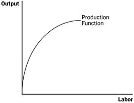
4.   We can draw a graph of the firm's production function by plotting the level of labor (x-axis) against the level of output (y-axis).

NOTE!!!!  I will do a simple example in this study guide.  Our in class assignments were more complex and included specialization.  These only have crowding.

a.   The slope of the production function measures marginal product.

b.   Diminishing marginal product can be seen from the fact that the slope falls as the amount of labor used increases.

B.   From the Production Function to the Total-Cost Curve

1.   We can draw a graph of the firm's total cost curve by plotting the level of output (x-axis) against the total cost of producing that output (y-axis).

a.   The total cost curve gets steeper and steeper as output rises.

III. The Various Measures of Cost

1.   Definition of fixed costs:

2.   Definition of variable costs:

C.   Average and Marginal Cost

1.   Definition of average total cost:

2.   Definition of average fixed cost:

3.   Definition of average variable cost:

4.   Definition of marginal cost:

5.   Average total cost tells us the cost of a typical unit of output and marginal cost tells us the cost of an additional unit of output.

D.   Cost Curves and Their Shapes

1.   Rising Marginal Cost

a.   This occurs because of diminishing marginal product.

b.   At a low level of output, there are few workers and a lot of idle equipment. But as output increases, the coffee shop gets crowded and the cost of producing another unit of output becomes high.

2.   U-Shaped Average Total Cost

a.   Average total cost is the sum of average fixed cost and average variable cost.                                         

b.   AFC declines as output expands and AVC typically increases as output expands. AFC is high when output levels are low. As output expands, AFC declines pulling ATC down. As fixed costs get spread over a large number of units, the effect of AFC on ATC falls and ATC begins to rise because of diminishing marginal product.

3.   The Relationship between Marginal Cost and Average Total Cost

a.   Whenever marginal cost is less than average total cost, average total cost is falling. Whenever marginal cost is greater than average total cost, average total cost is rising.

b.   The marginal-cost curve crosses the average-total-cost curve at minimum average total cost.

4.   Typical Cost Curves

a.   Marginal cost eventually rises with output.

b.   The average-total-cost curve is U-shaped.

c.    Marginal cost crosses average total cost at the minimum of average total cost.

   Definition of marginal revenue: the change in total revenue from an additional unit sold.

II.   Profit Maximization and the Competitive Firm's Supply Curve

  The Marginal-Cost Curve and the Firm's Supply Decision

1.   Cost curves have special features that are important for our analysis.

a.   The marginal-cost curve is upward sloping.

b.   The average-total-cost curve is U-shaped.

c.    The marginal-cost curve crosses the average-total-cost curve at the minimum of average total cost.

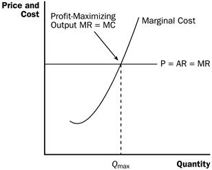
2.   Marginal and average revenue can be shown by a horizontal line at the market price.

3.   To find the profit-maximizing level of output, we can follow the same rules that we discussed above.

a.   If marginal revenue is greater than the marginal cost, the firm should increase its output.

b.   If marginal cost is greater than marginal revenue, the firm should decrease its output.

c.    At the profit-maximizing level of output, marginal revenue and marginal cost are exactly equal.

4.   These rules apply not only to competitive firms, but to firms with market power as well.

C.   The Firm's Short-Run Decision to Shut Down

1.   In certain circumstances, a firm will decide to shut down and produce zero output.

2.   There is a difference between a temporary shutdown of a firm and an exit from the market.

a.   A shutdown refers to a short-run decision not to produce anything during a specific period of time because of current market conditions.

b.   Exit refers to a long-run decision to leave the market.

c.    One important difference is that, when a firm shuts down temporarily, it still must pay fixed costs. If a firm exits the industry in the long run, it has no costs.

3.   If a firm shuts down, it will earn no revenue and will have only fixed costs (no variable costs).

4.   Therefore, a firm will shut down if the revenue that it would get from producing is less than its variable costs of production:

Shut down if TR < VC.

5.   Because TR = P x Q and VC = AVC x Q, we can rewrite this condition as:

Shut down if P < AVC.

6.   We now can tell exactly what the firm will do to maximize profit (or minimize loss).

a.   If the price is less than average variable cost, the firm will produce no output.

b.   If the price is above average variable cost, the firm will produce the level of output where marginal revenue (price) is equal to marginal cost.

7.   Therefore, the competitive firm's short-run supply curve is the portion of its marginal revenue curve that lies above average variable cost.

8.   Spilt Milk and Other Sunk Costs

a.   Definition of sunk cost: a cost that has been committed and cannot be recovered.

b.   Once a cost is sunk, it is no longer an opportunity cost.

c.    Because nothing can be done about sunk costs, you should ignore them when making decisions.

D.   The Firm's Long-Run Decision to Exit or Enter a Market

1.   If a firm exits the market, it will earn no revenue, but it will have no costs as well.

2.   Therefore, a firm will exit if the revenue that it would earn from producing is less than its total costs:

Exit if TR < TC.

3.   Because TR = P x Q and TC = ATC x Q, we can rewrite this condition as:

Exit if P < ATC.

4.   A firm will enter an industry when there is profit potential, so this must mean that a firm will enter if revenues will exceed costs:

Enter if P > ATC. 

5.   Because, in the long run, a firm will remain in a market only if P ≥ ATC, the firm's long-run supply curve will be its marginal cost curve above ATC.

E.   Measuring Profit in Our Graph for the Competitive Firm

1.   Recall that Profit = TR −TC.

2.   Because TR = P x Q and TC = ATC x Q, we can rewrite this equation:

Profit = (P – ATC) x Q.

3.   Using this equation, we can measure the amount of profit (or loss) at the firm's profit-maximizing level of output (or loss-minimizing level of output).

III. The Supply Curve in a Competitive Market

A.   The Short Run: Market Supply with a Fixed Number of Firms

1.   Example: a market with 1,000 identical firms.

2.   Each firm's short-run supply curve is its marginal cost curve above average variable cost.

3.   To get the market supply curve, we add the quantity supplied by each firm in the market at every given price.

B.   The Long Run: Market Supply with Entry and Exit

1.   If firms in an industry are earning profit, this will attract new firms.

a.   The supply of the product will increase (the supply curve will shift to the right).

b.   The price of the product will fall and profit will decline.

2.   If firms in an industry are incurring losses, firms will exit.

a.   The supply of the product will decrease (the supply curve will shift to the left).

b.   The price of the product will rise and losses will decline.

3.   At the end of this process of entry or exit, firms that remain in the market must be earning zero economic profit.

4.   Because Profit = TR –TC, profit will only be zero when:

TR = TC.

5.   Because TR = P x Q and TC = ATC x Q, we can rewrite this as:

P = ATC.

6.   Therefore, the process of entry or exit ends only when price and average total cost become equal.

7.   This implies that the long-run equilibrium of a competitive market must have firms operating at their efficient scale.