
I. The
Elasticity of Demand
A. Definition of elasticity:
B. The Price
Elasticity of Demand and Its Determinants
1. Definition of price elasticity of demand:
2.
Determinants of the Price Elasticity of Demand
a.
Availability of Close Substitutes: the more substitutes a good has, the more
elastic its demand.
b. Necessities
versus Luxuries: necessities are more price inelastic.
c.
Definition of the market: narrowly defined markets (ice cream) have more elastic
demand than broadly defined markets (food).
d. Time
Horizon: goods tend to have more elastic demand over longer time horizons.
C. Computing
the Price Elasticity of Demand
1. Formula

![]()
2. Example: the
price of ice cream rises by 10% and quantity demanded falls by 20%.
Price
elasticity of demand = (20%)/(10%) = 2
3. Because
there is an inverse relationship between price and quantity demanded (the price
of ice cream rose by 10% and the quantity demanded fell by 20%), the price
elasticity of demand is sometimes reported as a negative number. We will ignore
the minus sign and concentrate on the absolute value of the elasticity.
D. The Midpoint
Method:
1. Because we
use percentage changes in calculating the price elasticity of demand, the
elasticity calculated by going from one point to another on a demand curve will
be different from an elasticity calculated by going from the second point to the
first. This difference arises because the percentage changes are calculated
using a different base.
a. A way
around this problem is to use the midpoint method.
b. Using the
midpoint method involves calculating the percentage change in either price or
quantity demanded by dividing the change in the variable by the midpoint between
the initial and final levels rather than by the initial level itself.
c.
Example: the price rises from $4 to $6 and quantity demanded falls from 120 to
80.
% change in price = (6
- 4)/5 × 100% = 40%
% change in quantity
demanded = (120-80)/100 = 40%
price elasticity of
demand = 40/40 = 1

E. The Variety
of Demand Curves

1.
Classification of Elasticity
a. When the
price elasticity of demand is greater than one, demand is defined to be elastic.
b. When the
price elasticity of demand is less than one, the demand is defined to be
inelastic.
c. When
the price elasticity of demand is equal to one, the demand is said to have unit
elasticity.
2. In general,
the flatter the demand curve that passes through a given point, the more elastic
the demand.
3.
Extreme Cases
a. When the
price elasticity of demand is equal to zero, the demand is perfectly inelastic
and is a vertical line.
b. When the
price elasticity of demand is infinite, the demand is perfectly elastic and is a
horizontal line.

![]()
F.
Total Revenue and the Price Elasticity of Demand
1. Definition
of total revenue: the amount paid
by buyers and received by sellers of a good, computed as the price of the good
times the quantity sold.
2. If demand is
inelastic, the percentage change in price will be greater than the percentage
change in quantity demanded.
a. If price
rises, quantity demanded falls, and total revenue will rise (because the
increase in price will be larger than the decrease in quantity demanded).
b. If price
falls, quantity demanded rises, and total revenue will fall (because the fall in
price will be larger than the increase in quantity demanded).
3. If demand is
elastic, the percentage change in quantity demanded will be greater than the
percentage change in price.
a. If price
rises, quantity demanded falls, and total revenue will fall (because the
increase in price will be smaller than the decrease in quantity demanded).
b. If price
falls, quantity demanded rises, and total revenue will rise (because the fall in
price will be smaller than the increase in quantity demanded).
G. Elasticity
and Total Revenue along a Linear Demand Curve

1. The slope of
a linear demand curve is constant, but the elasticity is not.
a. At points
with a low price and a high quantity demanded, demand is inelastic.
b. At points
with a high price and a low quantity demanded, demand is elastic.
2. Total
revenue also varies at each point along the demand curve.
I. Other
Demand Elasticities
II. The Elasticity of Supply--Again in the book, but not on the test. Focus on the HW problems.
III. Three Applications of
Supply, Demand, and Elasticity
A. Can Good
News for Farming Be Bad News for Farmers?
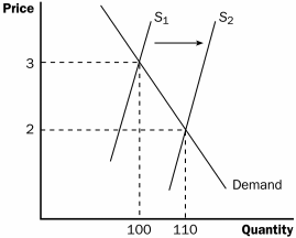
1. A new hybrid
of wheat is developed that is more productive than those used in the past. What
happens?
2. Supply
increases, price falls, and quantity demanded rises.
3. If demand is
inelastic, the fall in price is greater than the increase in quantity demanded
and total revenue falls.
4. If demand is
elastic, the fall in price is smaller than the rise in quantity demanded and
total revenue rises.
5. In practice,
the demand for basic foodstuffs (like wheat) is usually inelastic.
a. This means
less revenue for farmers.
b. Because
farmers are price takers, they still have the incentive to adopt the new hybrid
so that they can produce and sell more wheat.
c. This
may help explain why the number of farms has declined so dramatically over the
past two centuries.
d. This may
also explain why some government policies encourage farmers to decrease the
amount of crops planted.
B. Why Did OPEC
Fail to Keep the Price of Oil High?
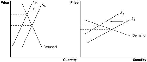
1. In the 1970s
and 1980s, OPEC reduced the amount of oil it was willing to supply to world
markets. The decrease in supply led to an increase in the price of oil and a
decrease in quantity demanded. The increase in price was much larger in the
short run than the long run. Why?
2. The demand
and supply of oil are much more inelastic in the short run than the long run.
The demand is more elastic in the long run because consumers can adjust to the
higher price of oil by carpooling or buying a vehicle that gets better mileage.
The supply is more elastic in the long run because non-OPEC producers will
respond to the higher price of oil by producing more.
C. Does Drug
Interdiction Increase or Decrease Drug-Related Crime?
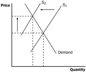
1. The federal
government increases the number of federal agents devoted to the war on drugs.
What happens?
a. The supply
of drugs decreases, which raises the price and leads to a reduction in quantity
demanded. If demand is inelastic, total expenditure on drugs (equal to total
revenue) will increase. If demand is elastic, total expenditure will fall.
b. Thus,
because the demand for drugs is likely to be inelastic, drug-related crime may
rise.
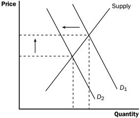
2. What happens
if the government instead pursued a policy of drug education?
a. The demand
for drugs decreases, which lowers price and quantity supplied. Total expenditure
must fall (because both price and quantity fall).
b. Thus, drug
education should not increase drug-related crime.
I. What
Are Costs?
A. Total
Revenue, Total Cost, and Profit
1. The goal of
a firm is to maximize profit.
2. Definition of total revenue:
![]()
3. Definition of total cost:
4. Definition of profit:
![]()
B. Costs as
Opportunity Costs
1. The cost of
something is what you give up to get it.
2. The costs of
producing an item must include all of the opportunity costs of inputs used in
production.
3. Total
opportunity costs include both implicit and explicit costs.
a. Definition of explicit costs:
b. Definition of implicit costs:
c. The
total cost of a business is the sum of explicit costs and implicit costs.
d. This is the
major way in which accountants and economists differ in analyzing the
performance of a business.
e. Accountants
focus on explicit costs, while economists examine both explicit and implicit
costs.
D. Economic Profit versus Accounting Profit
Definition of economic profit:
a. Economic
profit is what motivates firms to supply goods and services.
b. To
understand how industries evolve, we need to examine economic profit.
3. Definition of accounting profit:
4. If implicit
costs are greater than zero, accounting profit will always exceed economic
profit.
II. Production and Costs
A. The
Production Function
1. Definition of production function:
2. Example:
Caroline's cookie factory. The size of the factory is assumed to be fixed;
Caroline can vary her output (cookies) only by varying the labor used.
|
Number
of Workers |
Output |
Marginal
Product of Labor |
Cost of
Factory |
Cost of
Workers |
Total
Cost of Inputs |
|
0 |
0 |
--- |
$30 |
$0 |
$30 |
|
1 |
50 |
50 |
30 |
10 |
40 |
|
2 |
90 |
40 |
30 |
20 |
50 |
|
3 |
120 |
30 |
30 |
30 |
60 |
|
4 |
140 |
20 |
30 |
40 |
70 |
|
5 |
150 |
10 |
30 |
50 |
80 |
|
6 |
155 |
5 |
30 |
60 |
90 |
3. Definition of marginal product:

a. As the
amount of labor used increases, the marginal product of labor falls.
b. Definition
of diminishing marginal product:
4. We can draw
a graph of the firm's production function by plotting the level of labor (x-axis)
against the level of output (y-axis).
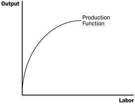
a. The slope
of the production function measures marginal product.
b. Diminishing
marginal product can be seen from the fact that the slope falls as the amount of
labor used increases.
B. From the
Production Function to the Total-Cost Curve
1. We can draw
a graph of the firm's total cost curve by plotting the level of output (x-axis)
against the total cost of producing that output (y-axis).
a. The total
cost curve gets steeper and steeper as output rises.
b. This
increase in the slope of the total cost curve is also due to diminishing
marginal product: As Helen increases the production of cookies, her kitchen
becomes overcrowded, and she needs a lot more labor.
III. The Various Measures
of Cost
Fixed and Variable
Costs
1. Definition of fixed costs:
2. Definition of variable costs:
![]()
3. Total cost is equal to
fixed cost plus variable cost.
|
Output |
Total
Cost |
Fixed
Cost |
Variable
Cost |
Average
Fixed Cost |
Average
Variable Cost |
Average
Total Cost |
Marginal
Cost |
|
0 |
$3.00 |
$3.00 |
$0 |
--- |
--- |
--- |
--- |
|
1 |
3.30 |
3.00 |
0.30 |
$3.00 |
$0.30 |
$3.30 |
$0.30 |
|
2 |
3.80 |
3.00 |
0.80 |
1.50 |
0.40 |
1.90 |
0.50 |
|
3 |
4.50 |
3.00 |
1.50 |
1.00 |
0.50 |
1.50 |
0.70 |
|
4 |
5.40 |
3.00 |
2.40 |
0.75 |
0.60 |
1.35 |
0.90 |
|
5 |
6.50 |
3.00 |
3.50 |
0.60 |
0.70 |
1.30 |
1.10 |
|
6 |
7.80 |
3.00 |
4.80 |
0.50 |
0.80 |
1.30 |
1.30 |
|
7 |
9.30 |
3.00 |
6.30 |
0.43 |
0.90 |
1.33 |
1.50 |
|
8 |
11.00 |
3.00 |
8.00 |
0.38 |
1.00 |
1.38 |
1.70 |
|
9 |
12.90 |
3.00 |
9.90 |
0.33 |
1.10 |
1.43 |
1.90 |
|
10 |
15.00 |
3.00 |
12.00 |
0.30 |
1.20 |
1.50 |
2.10 |
C. Average and
Marginal Cost
1. Definition of average total cost:
2. Definition of average fixed cost:
3. Definition
of average variable cost:
4. Definition of marginal cost:
![]()
5. Average
total cost tells us the cost of a typical unit of output and marginal cost tells
us the cost of an additional unit of output.
D. Cost Curves
and Their Shapes
1. Rising
Marginal Cost
a. This occurs
because of diminishing marginal product.
b. At a low
level of output, there are few workers and a lot of idle equipment. But as
output increases, the coffee shop gets crowded and the cost of producing another
unit of output becomes high.
2. U-Shaped
Average Total Cost
a. Average
total cost is the sum of average fixed cost and average variable cost.
![]()
b.
AFC declines as output expands and
AVC typically increases as output
expands. AFC is high when output
levels are low. As output expands, AFC
declines pulling ATC down. As fixed
costs get spread over a large number of units, the effect of
AFC on
ATC falls and
ATC begins to rise because of
diminishing marginal product.
c.
Definition of efficient scale:
the quantity of output that minimizes average total cost.
3. The
Relationship between Marginal Cost and Average Total Cost
a. Whenever
marginal cost is less than average total cost, average total cost is falling.
Whenever marginal cost is greater than average total cost, average total cost is
rising.
b. The
marginal-cost curve crosses the average-total-cost curve at minimum average
total cost (the efficient scale).
4. Typical Cost
Curves
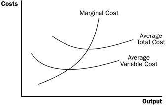
a. Marginal
cost eventually rises with output.
b. The
average-total-cost curve is U-shaped.
c. Marginal cost crosses average total cost at the minimum of average total cost.
IV. Costs in the
Short Run and in the Long Run
A. The division
of total costs into fixed and variable costs will vary from firm to firm.
B. Some costs
are fixed in the short run, but all are variable in the long run.
1. For example,
in the long run a firm could choose the size of its factory.
2. Once a
factory is chosen, the firm must deal with the short-run costs associated with
that plant size.
C. The long-run
average-total-cost curve lies along the lowest points of the short-run
average-total-cost curves because the firm has more flexibility in the long run
to deal with changes in production.
D. The long-run
average-total-cost curve is typically U-shaped, but is much flatter than a
typical short-run average-total-cost curve.
E. The length
of time for a firm to get to the long run will depend on the firm involved.
F. Economies
and Diseconomies of Scale
1. Definition of economies of scale:
2. Definition of diseconomies of scale:
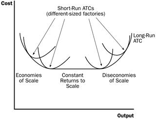
3. Definition of
constant returns to scale: