Untitled 2

EXTERNALITIES

You should understand:

what an externality is.

why externalities can make market outcomes inefficient. This is a very interesting point and has a big impact on taxing an externality.

how people can sometimes solve the problem of externalities on their own.

why private solutions to externalities sometimes do not work.

the various government policies aimed at solving the problem of externalities

KEY POINTS:

When a transaction between a buyer and seller directly affects a third party, that effect is called an externality. Negative externalities, such as pollution, cause the socially optimal quantity in a market to be less than the equilibrium quantity. Positive externalities, such as technology spillovers, cause the socially optimal quantity to be greater than the equilibrium quantity.

Those affected by externalities can sometimes solve the problem privately. For instance, when one business confers an externality on another business, the two businesses can internalize the externality by merging. Alternatively, the interested parties can solve the problem by signing a contract. According to the Coase theorem, if people can bargain without cost, then they can always reach an agreement in which resources are allocated efficiently. In many cases, however, reaching a bargain among the many interested parties is difficult, so the Coase theorem does not apply.

When private parties cannot adequately deal with external effects, such as pollution, the government often steps in. Sometimes the government prevents socially inefficient activity by regulating behavior. Other times it internalizes an externality using Pigouvian taxes. Another way to protect the environment is for the government to issue a limited number of pollution permits. The end result of this policy is largely the same as imposing Pigouvian taxes on polluters.

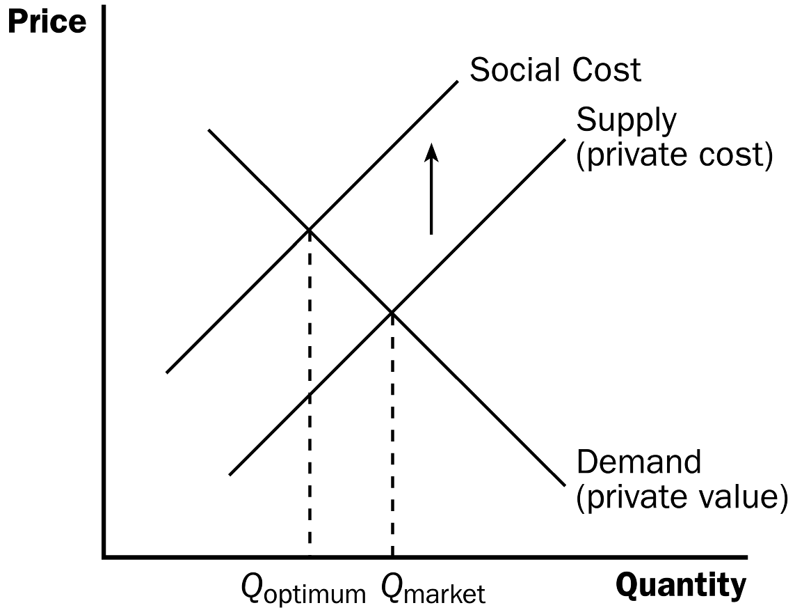
Negative Production Externality

_________________________________________________________________

Positive Consumption Externality

PUBLIC GOODS AND COMMON RESOURCES
You should understand:

the defining characteristics of public goods and common resources.

why private markets fail to provide public goods.

some of the important public goods in our economy.

why the cost–benefit analysis of public goods is both necessary and difficult.

why people tend to use common resources too much.

some of the important common resources in our economy

KEY POINTS:

Goods differ in whether they are excludable and whether they are rival. A good is excludable if it is possible to prevent someone from using it. A good is rival if one person’s enjoyment of the good prevents other people from enjoying the same unit of the good. Markets work best for private goods, which are both excludable and rival. Markets do not work as well for other types of goods.

Public goods are neither rival nor excludable. Examples of public goods include fireworks displays, national defense, and the creation of fundamental knowledge. Because people are not charged for their use of the public good, they have an incentive to free ride when the good is provided privately. Therefore, governments provide public goods, making their decision about the quantity based on cost–benefit analysis.

Common resources are rival but not excludable. Examples include common grazing land, clean air, and congested roads. Because people are not charged for their use of common resources, they tend to use them excessively. Therefore, governments try to limit the use of common resources.

Costs

You should understand:

what items are included in a firm’s costs of production.

the link between a firm’s production process and its total costs.

the meaning of average total cost and marginal cost and how they are related.

the shape of a typical firm’s cost curves.

the relationship between short-run and long-run costs.

KEY POINTS:

The goal of firms is to maximize profit, which equals total revenue minus total cost.

When analyzing a firm’s behavior, it is important to include all the opportunity costs of production. Some of the opportunity costs, such as the wages a firm pays its workers, are explicit. Other opportunity costs, such as the wages the firm owner gives up by working in the firm rather than taking another job, are implicit.

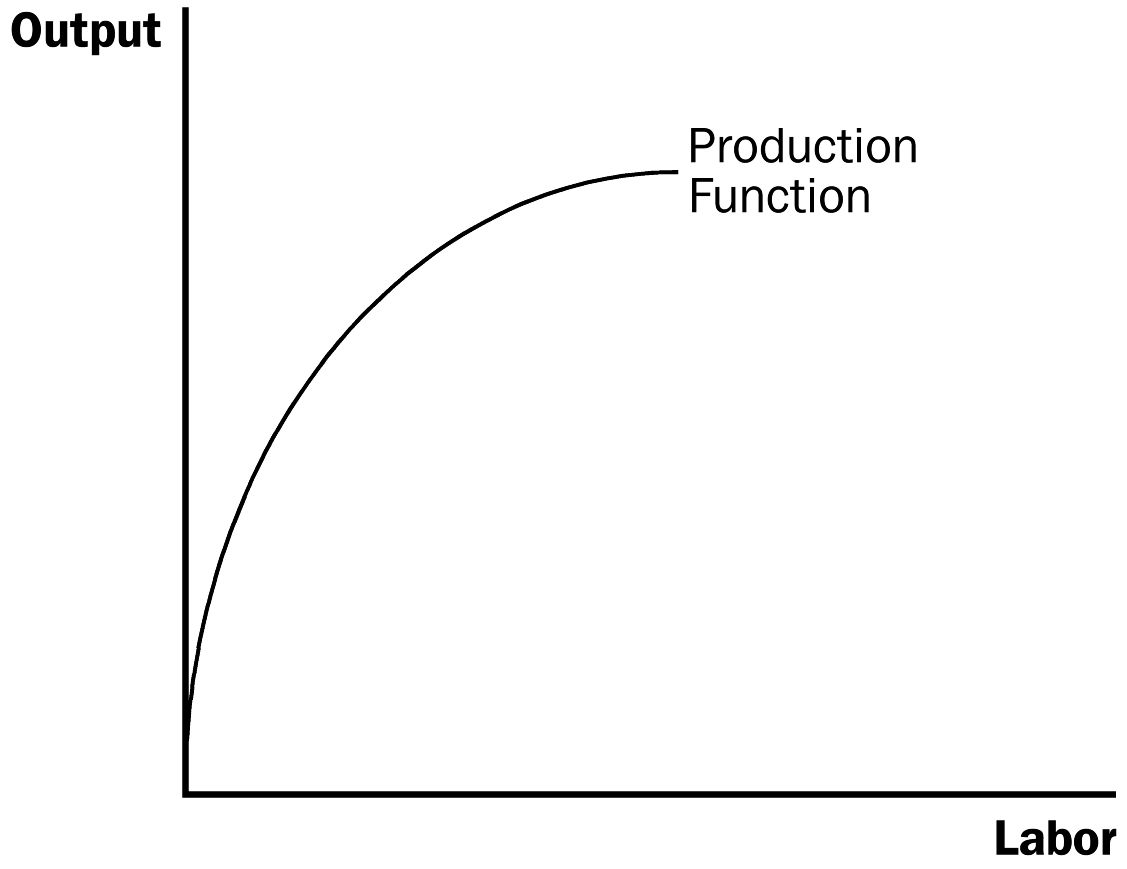
A firm’s costs reflect its production process. A typical firm’s production function gets flatter as the quantity of an input increases, displaying the property of diminishing marginal product. As a result, a firm’s total-cost curve gets steeper as the quantity produced rises.

A firm’s total costs can be divided between fixed costs and variable costs. Fixed costs are costs that do not change when the firm alters the quantity of output produced. Variable costs are costs that do change when the firm alters the quantity of output produced.

From a firm’s total cost, two related measures of cost are derived. Average total cost is total cost divided by the quantity of output. Marginal cost is the amount by which total cost would rise if output were increased by one unit.

When analyzing firm behavior, it is often useful to graph average total cost and marginal cost. For a typical firm, marginal cost rises with the quantity of output. Average total cost first falls as output increases and then rises as output increases further. The marginal-cost curve always crosses the average-total-cost curve at the minimum of average total cost.

A firm’s costs often depend on the time horizon being considered. In particular, many costs are fixed in the short run but variable in the long run. As a result, when the firm changes its level of production, average total cost may rise more in the short run than in the long run.

I. What Are Costs?

A. Total Revenue, Total Cost, and Profit

1. Goal of a firm: to maximize profit.

2. Definition of Tota1 Revenue: the amount a firm receives for the sale of its output.

3. Definition of Total Cost: the market value of the inputs a firm uses in production.

4. Definition of Profit: total revenue minus total cost.

B. Costs as Opportunity Costs

1. Principle #2: The cost of something is what you give up to get it.

2. The costs of producing an item must include all of the opportunity costs of inputs used in production.

3. Total opportunity costs include both implicit and explicit costs.

II. Production and Costs

A. The Production Function

1. Definition of Production Function: the relationship between quantity of inputs used to make a good and the quantity of output of that good.

2. Definition of Marginal Product: the increase in output that arises from an additional unit of input.

a. As the amount of labor used increases, the marginal product of labor falls.

Definition of Diminishing Marginal Product: the property whereby the marginal product of an input declines as the quantity of the input increases.

3. We can draw a graph of the firm’s production function by plotting the level of labor (x-axis) against the level of output (y-axis). This is the basic example.

a. The slope of the production function measures marginal product.

b. Diminishing marginal product can be seen from the fact that the slope falls as the amount of labor used increases.

B. From the Production Function to the Total-Cost Curve

1. We can draw a graph of the firm’s total cost curve by plotting the level of output (x-axis) against the total cost of producing that output (y-axis). Again, this is the basic graph.

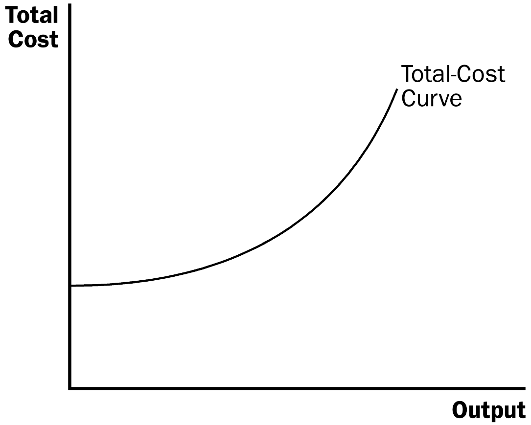
a. The total cost curve gets steeper and steeper as output rises.

b. This increase in the slope of the total cost curve is also due to diminishing marginal product: As Helen increases the production of cookies, she needs more labor and her kitchen becomes overcrowded.

III. The Various Measures of Cost

A. Fixed and Variable Costs

1. Definition of Fixed Costs: costs that do not vary with the quantity of output produced.

2. Definition of Variable Costs: costs that do vary with the quantity of output produced.

B. Average and Marginal Cost

1. Definition of Average Total Cost: total cost divided by the quantity of output.

2. Definition of Average Fixed Cost: fixed costs divided by the quantity of output.

3. Definition of Average Variable Cost: variable costs divided by the quantity of output.

4. Definition of Marginal Cost: the increase in total cost that arises from an extra unit of production.

5. Rising Marginal Cost

a. This occurs because of diminishing marginal product.

b. At a low level of output, there are few workers and a lot of idle equipment. But as output increases, the lemonade stand (or factory) gets crowded and the cost of producing another unit of output becomes high.

6. U-Shaped Average Total Cost

a. Average total cost is the sum of average fixed cost and average variable cost.

b. AFC declines as output expands and AVC increases as output expands. AFC is high when output levels are low. As output expands, AFC declines pulling ATC down. As fixed costs get spread over a large number of units, the effect of AFC on ATC falls and ATC begins to rise because of diminishing marginal product.

4. Typical Cost Curves

a. Marginal cost eventually rises with output.

b. The average total cost curve is U-shaped.

c. Marginal cost crosses average total cost at the minimum of the average total cost.