Untitled 1

SUPPLY and DEMAND

The previous midterm tested the introductory supply and and demand material. For this test, you should be able to use the graph.

ELASTICITY AND ITS APPLICATION

the meaning of the elasticity of demand.

what determines the elasticity of demand.

the concept of elasticity in three very different markets (the market for wheat, the market for oil, and the market for illegal drugs). We did not cover all of these examples, but they are good and worth reviewing.

KEY POINTS:

The price elasticity of demand measures how much the quantity demanded responds to changes in the price. Demand tends to be more elastic if the good is a luxury rather than a necessity, if close substitutes are available, if the market is narrowly defined, or if buyers have substantial time to react to a price change.

The price elasticity of demand is calculated as the percentage change in quantity demanded divided by the percentage change in price. If the elasticity is less than one, so that quantity demanded moves proportionately less than the price, demand is said to be inelastic. If the elasticity is greater than one, so that quantity demanded moves proportionately more than the price, demand is said to be elastic.

Total revenue, the total amount paid for a good, equals the price of the good times the quantity sold. For inelastic demand curves, total revenue rises as price rises. For elastic demand curves, total revenue falls as price rises.

Determinants of Price Elasticity of Demand

Necessities versus Luxuries: necessities are more price inelastic.

Availability of Close Substitutes: the more substitutes a good has, the more elastic its demand.

Definition of the Market: narrowly defined markets (ice cream) have more elastic demand than broadly defined markets (food).

Time Horizon: goods tend to have more elastic demand over longer time horizons.

Example: price of ice cream rises by 10% and quantity demanded falls by 20%.

Price elasticity of demand = (20%)/(10%) = 2

CAN YOU DO THE MIDPOINT METHOD!!!!!

When the elasticity is greater than one, the demand is considered to be elastic.

When the elasticity is less than one, the demand is considered to be inelastic.

Definition of Total Revenue: the amount paid by buyers and received by sellers of a good, computed as the price of the good times the quantity sold.

If demand is inelastic, the change in price will be greater than the change in quantity demanded.

If price rises, quantity demanded falls, and total revenue will rise (because the increase in price was larger than the decrease in quantity demanded).
If price falls, quantity demanded rises, and total revenue will fall (because the fall in price was larger than the increase in quantity demanded).

Example: Why Did OPEC Fail to Keep the Price of Oil High?

Example: Does Drug Interdiction Increase or Decrease Drug-Related Crime?

SUPPLY, DEMAND, AND GOVERNMENT POLICIES

the effects of government policies that place a ceiling on prices.

the effects of government policies that put a floor under prices.

how a tax on a good affects the price of the good and the quantity sold.

that taxes levied on buyers and taxes levied on sellers are equivalent.

how the burden of a tax is split between buyers and sellers.

KEY POINTS:

A price ceiling is a legal maximum on the price of a good or service. An example is rent control. If the price ceiling is below the equilibrium price, the quantity demanded exceeds the quantity supplied. Because of the resulting shortage, sellers must in some way ration the good or service among buyers.

A price floor is a legal minimum on the price of a good or service. An example is the minimum wage. If the price floor is above the equilibrium price, the quantity supplied exceeds the quantity demanded. Because of the resulting surplus, buyers’ demands for the good or service must in some way be rationed among sellers.

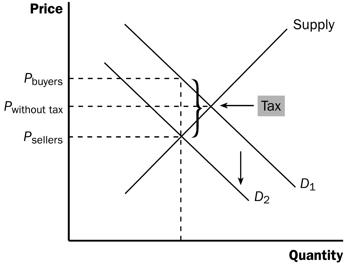
When the government levies a tax on a good, the equilibrium quantity of the good falls. That is, a tax shrinks the size of the market.

A tax on a good places a wedge between the price paid by buyers and the price received by sellers. When the market moves to the new equilibrium, buyers pay more for the good and sellers receive less for it. In this sense, buyers and sellers share the tax burden. the incidence of a tax does not depend on whether the tax is levied on buyers or sellers.

The incidence of a tax depends on the price elasticities of supply and demand. The burden tends to fall on the side of the market that is less elastic because that side of the market can respond less easily to the tax by changing the quantity bought or sold.

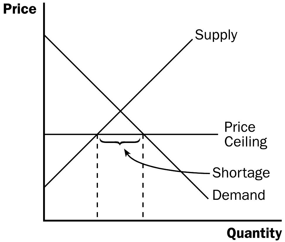
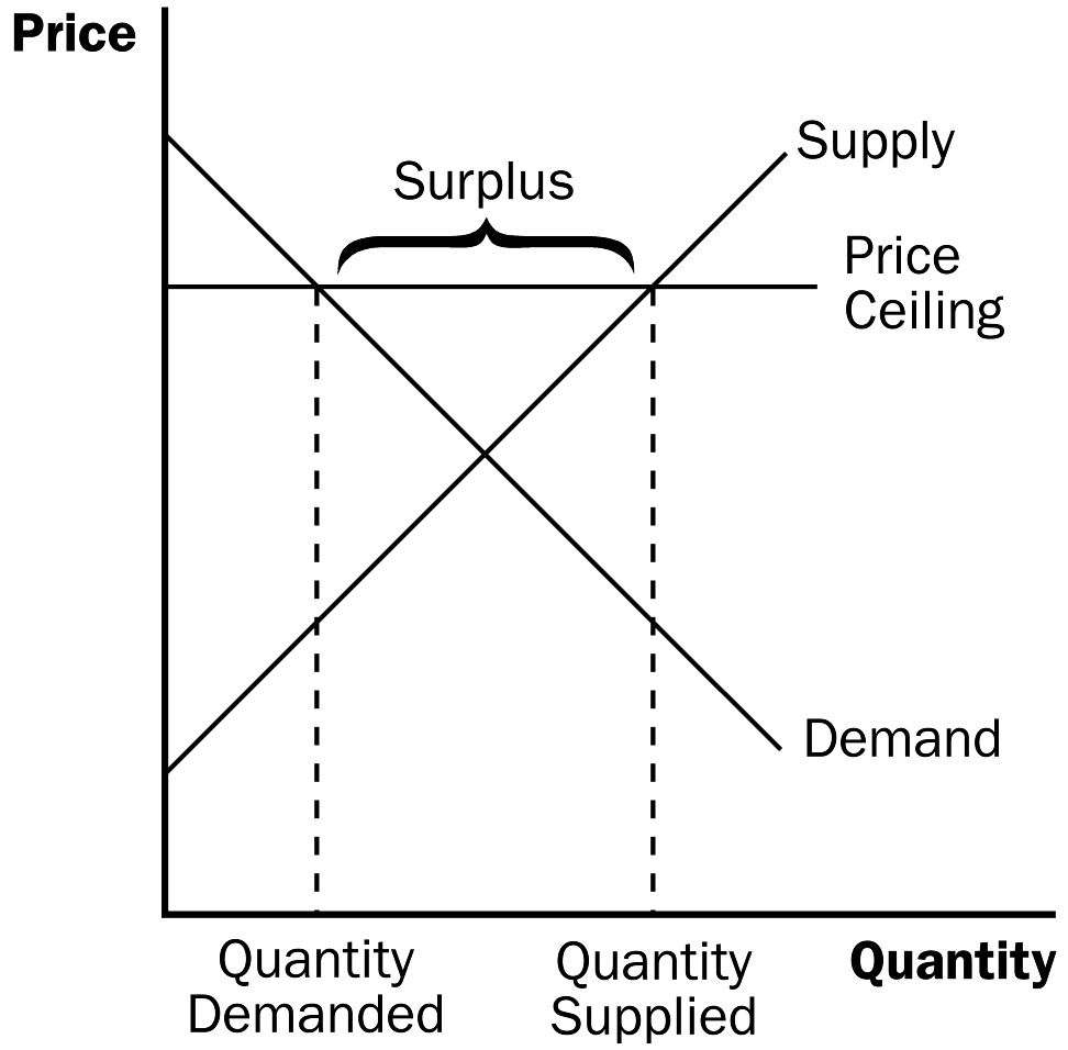
Oops! That should say price floor, but I cannot change it now!

Know at least one real world example of each policy!

CONSUMERS, PRODUCERS, AND EFFICIENCY OF MARKETS

You should understand:

the link between buyers’ willingness to pay for a good and the demand curve.

how to define and measure consumer surplus.

the link between sellers’ costs of producing a good and the supply curve.

how to define and measure producer surplus.

that the equilibrium of supply and demand maximizes total surplus in a market.

KEY POINTS:

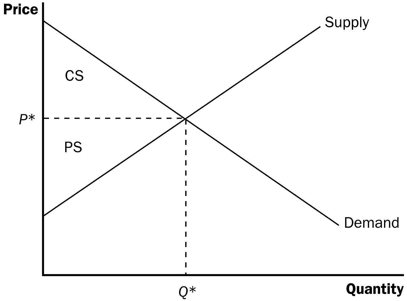
Consumer surplus equals buyers’ willingness to pay for a good minus the amount they actually pay for it, and it measures the benefit buyers get from participating in a market. Consumer surplus can be computed by finding the area below the demand curve and above the price.
Producer surplus equals the amount sellers receive for their goods minus their costs of production, and it measures the benefit sellers get from participating in a market. Producer surplus can be computed by finding the area below the price and above the supply curve.
An allocation of resources that maximizes the sum of consumer and producer surplus is said to be efficient. Policymakers are often concerned with the efficiency, as well as the equity, of economic outcomes.
The equilibrium of supply and demand maximizes the sum of consumer and producer surplus. That is, the invisible hand of the marketplace leads buyers and sellers to allocate resources efficiently.
Markets do not allocate resources efficiently in the presence of market failures such as market power or externalities.

APPLICATION: THE COSTS OF TAXATION

You should understand:

how taxes reduce consumer and producer surplus.

the meaning and causes of the deadweight loss from a tax.

why some taxes have larger deadweight losses than others.

how tax revenue and deadweight loss vary with the size of a tax.

KEY POINTS:

A tax on a good reduces the welfare of buyers and sellers of the good, and the reduction in consumer and producer surplus usually exceeds the revenue raised by the government. The fall in total surplus – the sum of consumer surplus, producer surplus, and tax revenue — is called the deadweight loss of the tax.

Taxes have deadweight losses because they cause buyers to consume less and sellers to produce less, and this change in behavior shrinks the size of the market below the level that maximizes total surplus. Because the elasticities of supply and demand measure how much market participants respond to market conditions, larger elasticities imply larger deadweight losses.

As a tax grows larger, it distorts incentives more, and its deadweight loss grows larger. Tax revenue first rises with the size of a tax. Eventually, however, a larger tax reduces tax revenue because it reduces the size of the market.

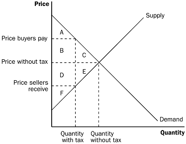
Welfare Before a Tax

a. Consumer surplus is equal to: A + B + C.

b. Producer surplus is equal to: D + E + F.

c. Total surplus is equal to: A + B + C + D + E + F.

Welfare with Tax

a. Consumer surplus is equal to: A.

b. Producer surplus is equal to: F.

c. Tax revenue is equal to: B + D.

d. Total surplus plus tax is equal to: A + B + D + F.

Definition of Deadweight Loss: the fall in total surplus that results from a market distortion, such as a tax.

When demand is relatively inelastic, the deadweight loss is small.

When demand is relatively elastic, the deadweight loss is large.

As taxes increase, the deadweight loss from the tax increases.

In fact, as taxes increase, the deadweight loss rises more quickly than the size of the tax.

Costs

You should understand:

what items are included in a firm’s costs of production.

the link between a firm’s production process and its total costs.

the meaning of average total cost and marginal cost and how they are related.

the shape of a typical firm’s cost curves.

the relationship between short-run and long-run costs.

KEY POINTS:

The goal of firms is to maximize profit, which equals total revenue minus total cost.

When analyzing a firm’s behavior, it is important to include all the opportunity costs of production. Some of the opportunity costs, such as the wages a firm pays its workers, are explicit. Other opportunity costs, such as the wages the firm owner gives up by working in the firm rather than taking another job, are implicit.

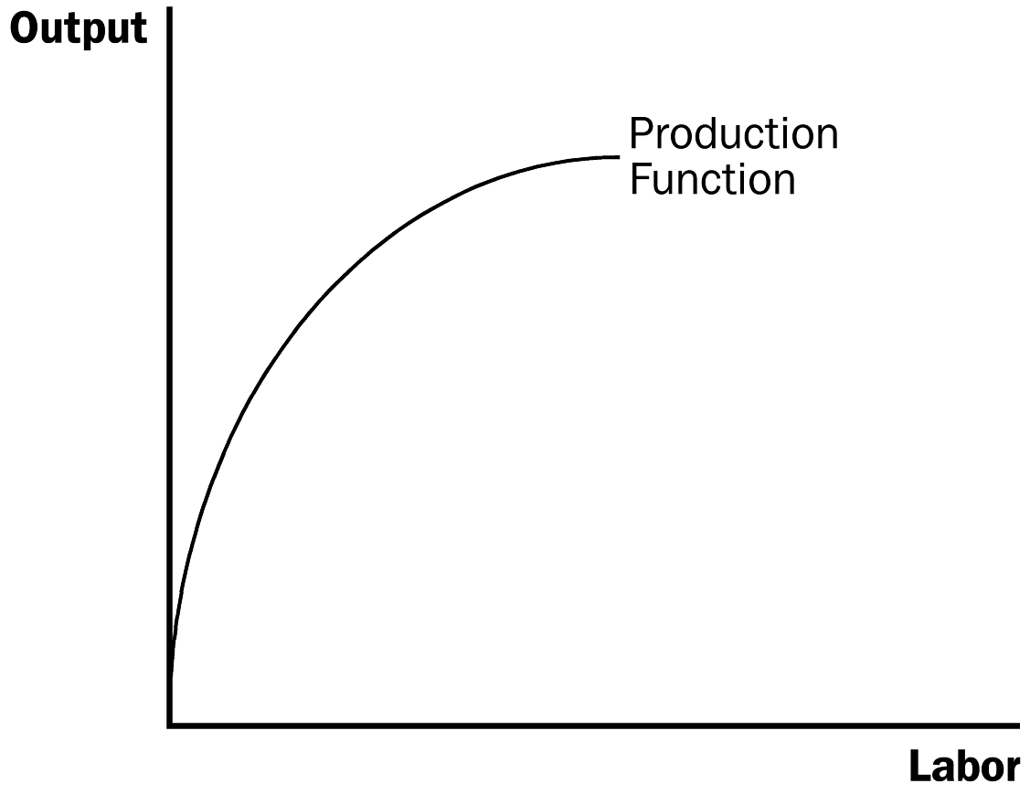
A firm’s costs reflect its production process. A typical firm’s production function gets flatter as the quantity of an input increases, displaying the property of diminishing marginal product. As a result, a firm’s total-cost curve gets steeper as the quantity produced rises.

A firm’s total costs can be divided between fixed costs and variable costs. Fixed costs are costs that do not change when the firm alters the quantity of output produced. Variable costs are costs that do change when the firm alters the quantity of output produced.

From a firm’s total cost, two related measures of cost are derived. Average total cost is total cost divided by the quantity of output. Marginal cost is the amount by which total cost would rise if output were increased by one unit.

When analyzing firm behavior, it is often useful to graph average total cost and marginal cost. For a typical firm, marginal cost rises with the quantity of output. Average total cost first falls as output increases and then rises as output increases further. The marginal-cost curve always crosses the average-total-cost curve at the minimum of average total cost.

A firm’s costs often depend on the time horizon being considered. In particular, many costs are fixed in the short run but variable in the long run. As a result, when the firm changes its level of production, average total cost may rise more in the short run than in the long run.

I. What Are Costs?

A. Total Revenue, Total Cost, and Profit

1. Goal of a firm: to maximize profit.

2. Definition of Tota1 Revenue: the amount a firm receives for the sale of its output.

3. Definition of Total Cost: the market value of the inputs a firm uses in production.

4. Definition of Profit: total revenue minus total cost.

B. Costs as Opportunity Costs

1. Principle #2: The cost of something is what you give up to get it.

2. The costs of producing an item must include all of the opportunity costs of inputs used in production.

3. Total opportunity costs include both implicit and explicit costs.

II. Production and Costs

A. The Production Function

1. Definition of Production Function: the relationship between quantity of inputs used to make a good and the quantity of output of that good.

2. Definition of Marginal Product: the increase in output that arises from an additional unit of input.

a. As the amount of labor used increases, the marginal product of labor falls.

Definition of Diminishing Marginal Product: the property whereby the marginal product of an input declines as the quantity of the input increases.

3. We can draw a graph of the firm’s production function by plotting the level of labor (x-axis) against the level of output (y-axis). This is the basic example.

a. The slope of the production function measures marginal product.

b. Diminishing marginal product can be seen from the fact that the slope falls as the amount of labor used increases.

B. From the Production Function to the Total-Cost Curve

1. We can draw a graph of the firm’s total cost curve by plotting the level of output (x-axis) against the total cost of producing that output (y-axis). Again, this is the basic graph.

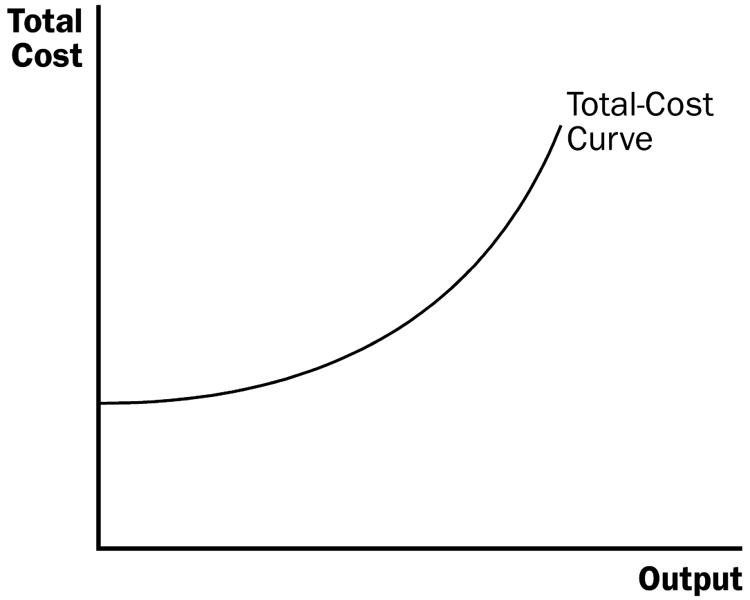
a. The total cost curve gets steeper and steeper as output rises.

b. This increase in the slope of the total cost curve is also due to diminishing marginal product: As Helen increases the production of cookies, she needs more labor and her kitchen becomes overcrowded.

III. The Various Measures of Cost

A. Fixed and Variable Costs

1. Definition of Fixed Costs: costs that do not vary with the quantity of output produced.

2. Definition of Variable Costs: costs that do vary with the quantity of output produced.

B. Average and Marginal Cost

1. Definition of Average Total Cost: total cost divided by the quantity of output.

2. Definition of Average Fixed Cost: fixed costs divided by the quantity of output.

3. Definition of Average Variable Cost: variable costs divided by the quantity of output.

4. Definition of Marginal Cost: the increase in total cost that arises from an extra unit of production.

5. Rising Marginal Cost

a. This occurs because of diminishing marginal product.

b. At a low level of output, there are few workers and a lot of idle equipment. But as output increases, the lemonade stand (or factory) gets crowded and the cost of producing another unit of output becomes high.

6. U-Shaped Average Total Cost

a. Average total cost is the sum of average fixed cost and average variable cost.

b. AFC declines as output expands and AVC increases as output expands. AFC is high when output levels are low. As output expands, AFC declines pulling ATC down. As fixed costs get spread over a large number of units, the effect of AFC on ATC falls and ATC begins to rise because of diminishing marginal product.

4. Typical Cost Curves

a. Marginal cost eventually rises with output.

b. The average total cost curve is U-shaped.

c. Marginal cost crosses average total cost at the minimum of the average total cost.