2.
A decline in productivity growth is the primary reason for the slowdown
in output growth in the United States since 1973. Productivity growth may have
declined because of deterioration in the legal and human environment, reduced
rates of technological innovation, and the effects of high oil prices. To some
extent the apparent decline in productivity may be due to measurement
difficulties.
3.
The rise in productivity growth in the 1990s occurred because of the
revolution in information and communications technologies (ICT). Not only were
there improvements in ICT, but also government regulations did not rein in the
growth of productivity in the United States, as they did in other countries,
such as those in Europe. In addition, intangible investment (research and
development, reorganization of firms, and worker training) allowed the ICT
improvements to boost productivity.
4.
A steady state is a situation in which the economy’s output per worker,
consumption per worker,
and capital stock per worker are constant.
5.
If there is no productivity growth, then output per worker, consumption
per worker, and capital per worker will all be constant in the long run. This
represents a steady state for the economy.
1. (a)
The destruction of some of a country’s capital stock in a war would have
no effect on the steady state, because there has been no change in s,
f, n, or d. Instead, k is reduced temporarily,
but equilibrium forces eventually drive k to the same steady-state value
as before.
(b)
Immigration raises n from n1 to n2
in Figure 6.3. The rise in n lowers steady-state k,
leading to a lower steady-state consumption per worker.
Figure 6.3
(c)
The rise in energy prices reduces the productivity of capital per worker.
This causes sf(k) to shift down from sf1(k)
to sf2(k) in
Figure 6.4. The result is a decline in steady-state k. Steady-state
consumption per worker falls for two reasons: (1) Each unit of capital has a
lower productivity, and (2) steady-state k is reduced.
Figure 6.4
(d)
A temporary rise in s has no effect on the steady-state
equilibrium.
(e)
The increase in the size of the labor force does not affect the growth
rate of the labor force, so there is no impact on the steady-state capital-labor
ratio or on consumption per worker. However, because a larger fraction of
the population is working, consumption per person increases.
2. (a)
Solow model
The rise in
capital depreciation shifts up the (n +
d)k line from (n
+ d1)k to (n
+ d2)k,
as shown in Figure 6.5. The equilibrium steady-state capital-labor ratio
declines. With a lower capital-labor ratio, output per worker is lower, so
consumption per worker is lower (using the assumption that the capital-labor
ratio is not so high that an increase in k will reduce consumption per
worker). There is no effect on the long-run growth rate of the total capital
stock, because in the long run the capital stock must grow at the same rate (n)
as the labor force grows, so that the capital-labor ratio is constant.
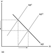
Figure 6.5
(b)
Endogenous growth model
In an
endogenous growth model, the growth rate of output is
DY/Y
=
sA - d, so the
rise in the deprecia-tion rate reduces the economy’s growth rate. Similarly, the
growth rate of capital equals DK/K
=
sA - d, which also
declines when the depreciation rate rises. Since consumption is a constant
fraction of output, its growth rate declines as well. So the increase in the
depreciation rate reduces the long-run growth rate of the capital stock, as well
as long-run capital, output, and consumption per worker.
5.
The initial level of the capital-labor ratio is irrelevant for the steady
state. Two economies that are identical except for their initial capital-labor
ratios will have exactly the same steady state.
Since the two economies must have the same growth rate at the steady
state, and since the economy with the higher current capital-labor ratio has
higher current output per worker, then the country with the lower current
capital-labor ratio must grow faster.
The answer holds true regardless of which country is in a steady state.
If the country with a higher initial capital-labor ratio is in a steady state at
capital-labor ratio k*, then the other country’s capital-labor
ratio will rise until it too equals k*. So the country with
the lower capital-labor ratio grows faster than the one with the higher
capital-labor ratio.
If the country with the lower initial capital-labor ratio is in a steady
state at capital-labor ratio k*, then the other country’s
capital-labor ratio is too high and it will decline until it equals k*.
So the country with the higher capital-labor ratio must grow more slowly than
the country with the lower capital-labor ratio. If the two countries are allowed
to trade with each other, then their convergence to the same capital-labor ratio
and output per worker will occur even faster.
2.
|
|
20 Years Ago |
Today |
Percent
Change |
|
Y |
1000 |
1300 |
30% |
|
K |
2500 |
3250 |
30% |
|
N |
500 |
575 |
15% |
(a)
DA/A
= DY/Y
- aK
DK/K
- aN DN/N
= 30%
- (0.3
´ 30%)
- 0.7
´ 15%
= 30%
- 9% -
10.5%
= 10.5%
Capital
growth contributed 9% (aK DK/K),
labor growth contributed 10.5% (aN
DN/N), productivity growth was 10.5%.
(b)
DA/A
= 30% - (0.5
´
30%) - (0.5
´ 15%)
= 30%
- 15% -
7.5%
= 7.5%
Capital
growth contributed 15% (aK DK/K),
labor growth contributed 7.5% (aN
DN/N), productivity growth was 7.5%.
3. (a)
|
Year |
K |
N |
Y |
K/N |
Y/N |
|
1 |
200 |
1000 |
617 |
0.20 |
0.617 |
|
2 |
250 |
1000 |
660 |
0.25 |
0.660 |
|
3 |
250 |
1250 |
771 |
0.20 |
0.617 |
|
4 |
300 |
1200 |
792 |
0.25 |
0.660 |
This
production function can be written in per-worker form since Y/N
= K.3N.7/N
= K.3/N.3
=
(K/N).3. Note that K/N is the same in
years 1 and 3, and so is Y/N. Also, K/N is the same
in years 2 and 4, and so is Y/N.
(b)
|
Year |
K |
N |
Y |
K/N |
Y/N |
|
1 |
200 |
1000 |
1231 |
0.20 |
1.231 |
|
2 |
250 |
1000 |
1316 |
0.25 |
1.316 |
|
3 |
250 |
1250 |
1574 |
0.20 |
1.259 |
|
4 |
300 |
1200 |
1609 |
0.25 |
1.341 |
This
production function can’t be written in per-worker form since
Y/N
=
K.3N.8/N =
K.3/N.2.
Note that K/N is the same in years 1 and 3, but Y/N
is not the same in these years. The same is true for years 2 and 4.
4.
To answer this problem, an approximate solution can be found by finding
the ratio GDP (2006)/GDP (1950), taking the natural logarithm of that ratio and
dividing by 56. This is the answer given in the table below.
|
|
Real GDP Per Capital |
Growth |
|||
|
1950 |
2006 |
|
Ratio |
Rate |
|
|
Australia |
7,412 |
24,343 |
|
3.28 |
2.1% |
|
Canada |
7,291 |
24,951 |
|
3.42 |
2.2% |
|
France |
5,186 |
21,809 |
|
4.21 |
2.6% |
|
Germany |
3,881 |
19,993 |
|
5.15 |
2.9% |
|
Japan |
1,921 |
22,462 |
|
11.69 |
4.4% |
|
Sweden |
6,739 |
24,204 |
|
3.59 |
2.2% |
|
United Kingdom |
6,939 |
23,013 |
|
3.32 |
2.1% |
|
United States |
9,561 |
31,049 |
|
3.25 |
2.1% |
Germany and Japan had the highest growth rates because damage from World
War II caused capital per worker to be lower than its steady-state level, and
thus output per worker was temporarily low.
5. (a)
sf(k) = (n +
d)k
0.3
´ 3k.5
= (0.05
+ 0.1)k
0.9k.5
= 0.15k
0.9/0.15
= k/k.5
6
= k.5
k
= 62
= 36
y
= 3k.5
= 3
´
6 = 18
c
= y
- (n
+
d)k = 18
- (0.15
´
36) = 12.6
(b) sf(k)
= (n +
d)k
0.4
´ 3k.5
= (0.05
+ 0.1)k
1.2k.5
= 0.15k
1.2/0.15
= k/k.5
8
= k.5
k
= 82
= 64
y
= 3k.5
= 3
´
8 = 24
c
= y
- (n
+
d)k = 24
- (0.15
´
64) = 14.4
(c) sf(k)
= (n +
d)k
0.3
´ 3k.5
= (0.08 + 0.1)k
0.9k.5
= 0.18k
0.9/0.18
= k/k.5
5
= k.5
k
= 52
= 25
y
= 3k.5
= 3
´
5 = 15
c
= y – (n
+
d)k = 15 - (0.18
´
25) = 10.5
(d)
sf(k) = (n
+ d)k
0.3
´
4k.5 = (0.05
+ 0.1)k
1.2k.5
= 0.15k
1.2/0.15
= k/k.5
8
= k.5
k
= 82
= 64
y
= 4k.5
= 4
´ 8 = 32
c
= y – (n
+
d)k = 32
- (0.15
´
64) = 22.4