5.    The MPN curve shows the marginal product of labor at each level of employment; it is the additional output obtained by adding one additional worker. It is related to the production function because the marginal product of labor is equal to the slope of the production function (where output is plotted against employment). The MPN curve is related to labor demand, because firms hire workers up to the point at which the real wage equals the marginal product of labor. So the labor demand curve is identical to the MPN curve, except that the vertical axis is the real wage instead of the marginal product of labor.

8.    Full-employment output is the level of output that firms supply when wages and prices in the economy have fully adjusted; in the classical model of the labor market, this occurs when the labor market is in equilibrium. When labor supply increases, full-employment output increases, as there is now more labor available to produce output. When a beneficial supply shock occurs, then the same quantities of labor and capital produce more output, so full-employment output rises. Furthermore,
a beneficial supply shock increases the demand for labor at each real wage and leads to an increase in the equilibrium level of employment, which also increases output.

12.  Frictional unemployment arises as workers and firms search to find matches. A certain amount of frictional unemployment is necessary, because it is not always possible to find the right match right away. For example, an unemployed banker may not want to take a job flipping hamburgers if he or she cannot find another banking job right away, because the match would be very poor. By remaining unemployed and continuing to search for a more suitable job, the banker is likely to make a better match. That will be better both for the banker (since the salary is likely to be higher) and for society as a whole (since the better match means greater productivity in the economy).

14.  The natural rate of unemployment is the rate of unemployment that prevails when output and employment are at their full-employment levels. The natural rate of unemployment is equal to the amount of frictional unemployment plus structural unemployment. Cyclical unemployment is the difference between the actual rate of unemployment and the natural rate of unemployment. When cyclical unemployment is negative, output and employment exceed their full-employment levels.

 1.    (a)  To find the growth of total factor productivity, you must first calculate the value of A in the production function. This is given by A = Y/(K^.3N^.7). The growth rate of A can then be
calculated as

[(A_{year 2} – A_{year 1})/A_{year 1}] ´ 100%. The result is:

        (b)  Calculate the marginal product of labor by seeing what happens to output when you add 1.0 to N; call this Y₂, and the original level of output Y₁. [A more precise method is to take the derivative of output with respect to N; dY/dN = 0.7A(K/N)^.3. The result is the same (rounded).]

 5.    (a)  If the lump-sum tax is increased, there’s an income effect on labor supply, not a substitution effect (since the real wage isn’t changed). An increase in the lump-sum tax reduces a worker’s wealth, so labor supply increases.

        (b)  If T = 35, then NS = 22 + 12w + (2 ´ 35) = 92 + 12 w. Labor demand is given by w = MPN =
309 – 2N, or 2N = 309 – w, so N = 154.5 – w/2. Setting labor supply equal to labor demand gives 154.5 – w/2 = 92 + 12w, so 62.5 = 12.5w, thus w = 62.5/12.5 = 5. With w = 5, N = 92 + (12 ´ 5) = 152.

        (c)  Since the equilibrium real wage is below the minimum wage, the minimum wage is binding. With w = 7, N = 154.5 – 7/2 = 151.0. Note that NS = 92 + (12 ´ 7) = 176, so NS > N and there is unemployment.

2.     (a)  An increase in the number of immigrants increases the labor force, increasing employment and increasing full-employment output.

        (b)  If energy supplies become depleted, this is likely to reduce productivity, because energy is a factor of production. So the reduction in energy supplies reduces full-employment output.

        (c)  This one could be interpreted in different ways and I was flexible when grading.  In general, better education raises productivity and output; therefore, companies will increase labor demand.  You could, however, make the argument that the change in education has a future effect and not a current effect.  In this case companies will not adjust their demand, but individuals will adjust based on anticipated future increases in labor demand.  That result would give a decrease in labor supply.

        (d)  This reduction in the capital stock reduces full-employment output (although it may very well increase welfare).

4.     (a)  The increased value of Helena’s home increases her wealth. The rise in wealth leads to an income effect that leads Helena to reduce her labor supply.

        (b)  This question was too labor economics, but we know that labor supply curve slopes upward except in extreme cases.  We should expect her supply of labor to increase.  The complete answer would be: the permanent rise in Helena’s real wage gives rise to offsetting income and substitution effects. The income effect of the higher wage reduces Helena’s labor supply, but the substitution effect increases it. So the result is theoretically ambiguous.

        (c)  The temporary income tax surcharge is equivalent to a temporary reduction in the real wage, which reduces current labor supply, assuming that the income effect is smaller than the substitution effect.

5.    This is a difficult problem and I will go through it slowly in class.  When government purchases increase temporarily, consumers see that higher taxes will be required in the future to pay off the deficit. They reduce both current consumption and future consumption, but current consumption declines by less than the amount of the government purchases. Since national saving is output minus desired consumption minus government purchases, and government purchases have increased more than current desired consumption has decreased, national saving declines at a given real interest rate.

       In the case of a lump-sum tax increase, consumers have higher taxes today, but lower taxes in the future. If consumers take this into account, current desired consumption is unchanged, and since output and government purchases didn’t change, desired national saving is unchanged as well. This is the case of Ricardian equivalence, and is controversial because consumers may not understand that higher taxes today imply lower future taxes. As a result, they may reduce desired consumption today, increasing desired national saving.

8.    Gross investment represents the total purchase or construction of new capital goods that takes place during a period. Net investment is gross investment minus the depreciation on existing capital. Thus net investment is the overall increase in the capital stock. Yes, it is possible for gross investment to be positive when net investment is negative. This occurs whenever gross investment is less than the amount of depreciation (and, in fact, happened in the United States during World War II).

2.     (a)  This chart shows the MPK^f as the increase in output from adding another fabricator:

        (b)  uc = (r + d)p_K = (0.12 + 0.20)$100 = $32. HHHHC should buy two fabricators, since at two fabricators, MPK^f = 50 > 32 = uc.  But at three fabricators, MPK^f = 30 < 32 = uc. You want to add fabricators only if the future marginal product of capital exceeds the user cost of capital. The MPK^f of the third fabricator is less than its user cost, so it should not be added.

        (c)  When r = 0.08, uc = (0.08 + 0.20)$100 = $28. Now they should buy three fabricators, since MPK^f = 30 > 28 = uc for the third fabricator and MPK^f = 15 < 28 = uc for the fourth fabricator.

        (d)  With taxes, they should add additional fabricators as long as (1 – t)MPK^f > uc. Since t = 0.4,
1 – t = 0.6. They should buy just one fabricator, since (1 – t)MPK^f = 0.6 ´ 100 = 60 > 32 = uc. They shouldn’t buy two, since then (1 – τ)MPK^f = 0.6 ´ 50 = 30 < 32 = uc.

        (e)  When output doubles, the MPK^f doubles as well. At r = 0.12, they should buy three fabricators, since then MPK^f = 60 > 32 = uc; they shouldn’t buy four, since then MPK^f = 30 < 32 = uc.

       At r = 0.08, they should buy four fabricators, since then MPK^f = 30 > 28 = uc; they shouldn’t buy five, since then MPK^f = 20 < 28 = uc.

6.     (a)  S^d = Y – C^d – G

= Y – (3600 – 2000r + 0.1Y) – 1200

= –4800 + 2000r + 0.9Y

(b)  (1) Using Eq. (4.7): Y = C^d + I^d + G

Y = (3600 – 2000r + 0.1Y) + (1200 – 4000r) + 1200

= 6000 – 6000r + 0.1Y

So 0.9Y = 6000 – 6000r

At full employment, Y = 6000. Solving 0.9 ´ 6000 = 6000 – 6000r, we get r = 0.10.

             (2) Using Eq. (4.8):

S^d = I^d

–4800 + 2000r + 0.9Y = 1200 – 4000r

0.9Y = 6000 – 6000r

When Y = 6000, r = 0.10.

So we can use either Eq. (4.7) or (4.8) to get to the same result.

        (c)  When G = 1440, desired saving becomes S^d = Y – C^d – G = Y – (3600 – 2000r + 0.1Y) – 1440 =
 –5040 + 2000r + 0.9Y. S^d is now 240 less for any given r and Y; this shows up as a shift in the S^d line from S¹ to S² in Figure 4.3.

Figure 4.3

Setting S^d = I^d, we get:

–5040 + 2000r + 0.9Y = 1200 – 4000r

6000r + 0.9Y = 6240

 1.    (a)  As Figure 4.5 shows, the shift to the right in the saving curve from S¹ to S² causes saving and investment to increase and the real interest rate to decrease.

Figure 4.5

        (b)  This is really just a transfer from the general population to veterans. The effect on saving depends on whether the marginal propensity to consume (MPC) of veterans differs from that of the general population. If there is no difference in MPCs, there will be no shift of the saving curve; neither investment nor the real interest rate is affected. If the MPC of veterans is higher than the MPC of the general population, then desired national saving declines and the saving curve shifts to the left; the real interest rate rises and investment declines. If the MPC of veterans is lower than that of the general population, the saving curve shifts to the right; the real interest rate declines and investment rises.

        However, must of you approached this problem in a more basic fashion.  You explored an increase in taxes.  If that is the case we can talk about Ricardian Equivalence or state that an increase in taxes will cause savings to rise and; therefore, investment will rise and real interest rates will fall.    

        (c)  The investment tax credit encourages investment, shifting the investment curve from I¹ to I² in Figure 4.6. Saving and investment increase, as does the real interest rate.

Figure 4.6

        (d)  The increase in expected future income decreases current desired saving, as people increase desired consumption immediately. The rise of the future marginal productivity of capital shifts the investment curve to the right. The result, as shown in Figure 4.7, is that the real interest rate rises, with ambiguous effects on saving and investment.

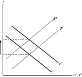
Figure 4.7