Untitled 1

1. (a) To find the growth of total factor productivity, you must first calculate the value of A in the production function. This is given by A  Y/(K^.3N^.7). The growth rate of A can then be
calculated as

[(A_{year 2} – A_{year
1})/A_{year 1}] ´ 100%. The result is:

	A	% increase in A
1960	12.484	—
1970	14.701	17.8%
1980	15.319	4.2%
1990	17.057	11.3%
2000	19.565	14.7%

(b) Calculate the marginal product of labor by seeing what happens to output when you add 1.0 to N; call this Y₂, and the original level of output Y₁. [A more precise method is to take the derivative of output with respect to N; dY/dN  0.7A(K/N)^.3. The result is the same (rounded).]

	Y₁	Y₂	MPN
1960	2502	2529	27
1970	3772	3805	33
1980	5162	5198	36
1990	7113	7155	42
2000	9817	9867	50

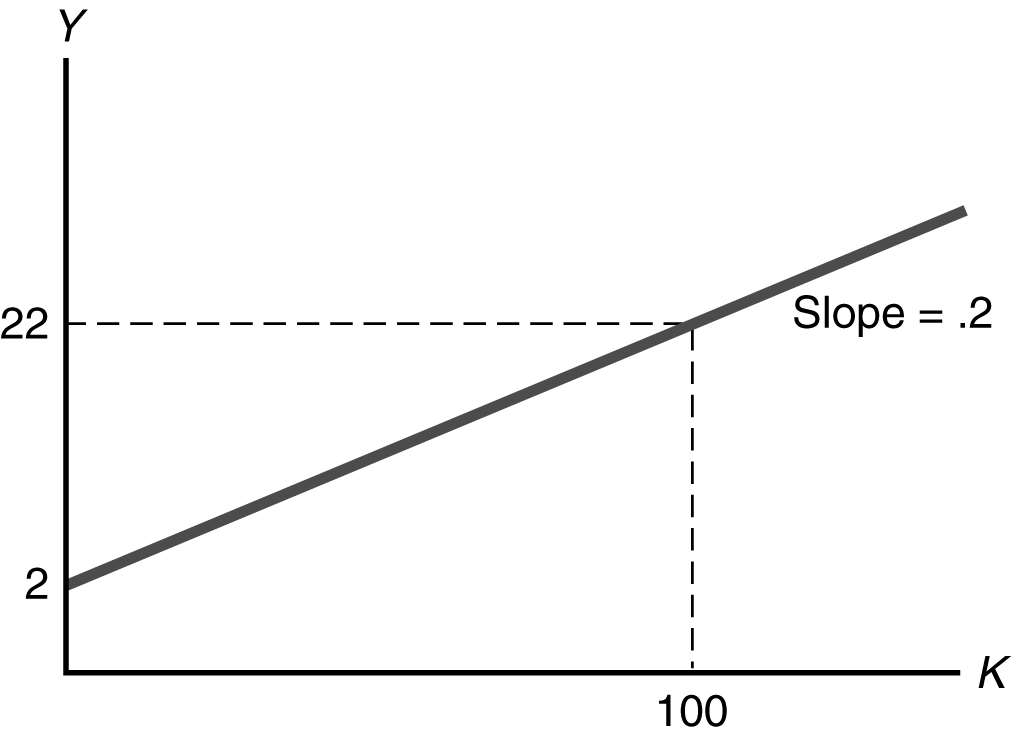
2. (a) The MPK is 0.2, because for each additional unit of capital, output increases by 0.2 units. The slope of the production function line is 0.2. There is no diminishing marginal productivity of capital in this case, because the MPK is the same regardless of the level of K. This can be seen in figure because the production function is a straight line.

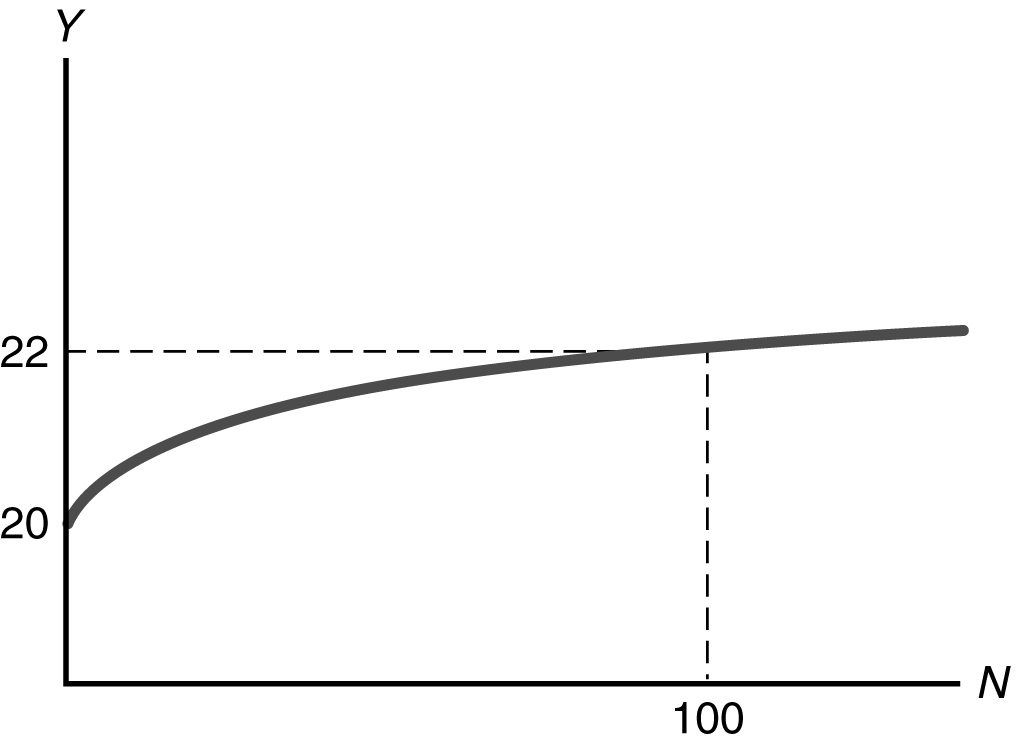
(b) When N is 100, output is Y  0.2(100  100^.5)  22. When N is 110, Y is 22.0976. So the MPN for raising N from 100 to 110 is (22.0976 – 22)/10  0.00976. When N is 120, Y is 22.1909. So the MPN for raising N from 110 to 120 is (22.1909 – 22.0976)/10  0.00933. This shows diminishing marginal productivity of labor because the MPN is falling as N increases. In figure this is shown as a decline in the slope of the production function as N increases.

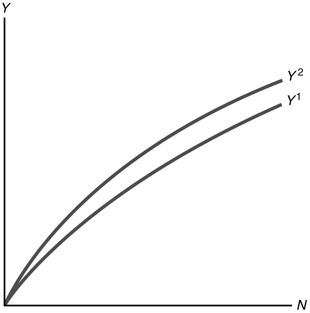
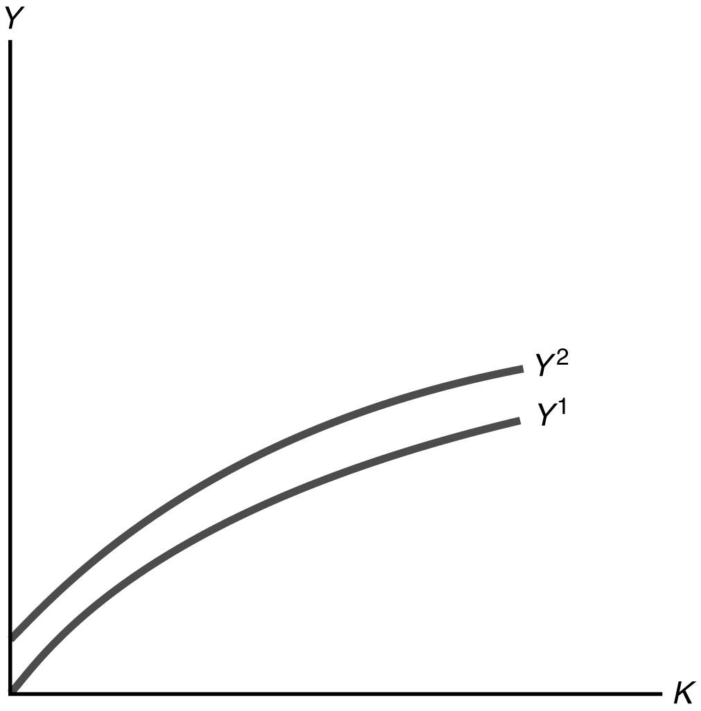
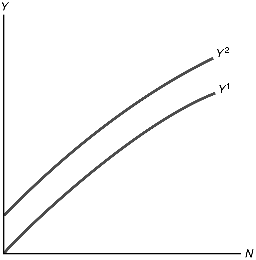
1. (a) See Figures

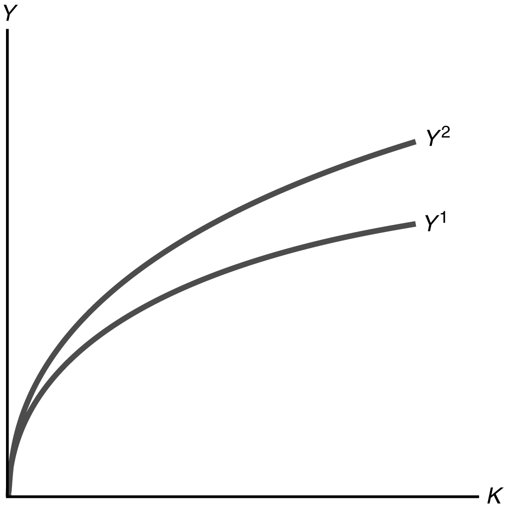
(b) In the initial situation, capital K₁ and labor N₁ produce output Y₁; when productivity rises they produce output 1.1 Y₁. Suppose that a small increase in capital to K₂ with labor left at N₁ produces output Y₂ in the initial situation. Then it produces 1.1 Y₂ when productivity rises by 10%. The marginal product of capital (MPK) in the initial situation is (Y₂ – Y₁)/(K₂ – K₁); when productivity rises the new MPK is (1.1 Y₂ – 1.1 Y₁)/(K₂ – K₁)  1.1 (Y₂ – Y₁)/(K₂ – K₁). So the new MPK is 10% higher than the old MPK.

This argument is completely symmetric, so it holds for MPN as well. If you substitute N for K everywhere and follow the same steps, you will show that the new MPN is 10% higher than the old MPN.

(c) Yes, it is possible for a beneficial productivity shock to leave the MPK and MPN unchanged. This could happen only if the shock was additive—that is, if it shifted the whole production function upward, but did not affect its slope at any point. In Figures this is shown as a shift up in the production function, leaving the slope unchanged. This, however, requires a combination of factors to get this result.

Figure 3.15

Figure 3.16

4. A steady state is a situation in which the economy’s output per worker, consumption per worker,
and capital stock per worker are constant.

5. If there is no productivity growth, then output per worker, consumption per worker, and capital per worker will all be constant in the long run. This represents a steady state for the economy.

6. The statement is false. Increases in the capital-labor ratio increase consumption per worker in the steady state only up to a point. If the capital-labor ratio is too high, then consumption per worker may decline due to diminishing marginal returns to capital, and the need to divert much of output to maintaining the capital-labor ratio.

7. (a) An increase in the saving rate increases long-run living standards, as higher saving allows for more investment and a larger capital stock.

(b) An increase in the population growth rate reduces long-run living standards, as more output must be used to equip the larger number of new workers with capital, leaving less output available to increase consumption or capital per worker.

(c) A one-time increase in productivity increases living standards directly, by increasing output, and indirectly, since by raising incomes it also raises saving and the capital stock.

3. (a)

Year	K	N	Y	K/N	Y/N
1	200	1000	617	0.20	0.617
2	250	1000	660	0.25	0.660
3	250	1250	771	0.20	0.617
4	300	1200	792	0.25	0.660

This production function can be written in per-worker form since Y/N  K^.3N^.7/N  K^.3/N^.3 
(K/N)^.3. Note that K/N is the same in years 1 and 3, and so is Y/N. Also, K/N is the same in years 2 and 4, and so is Y/N.

(b)

Year	K	N	Y	K/N	Y/N
1	200	1000	1231	0.20	1.231
2	250	1000	1316	0.25	1.316
3	250	1250	1574	0.20	1.259
4	300	1200	1609	0.25	1.341

This production function can’t be written in per-worker form since Y/N  K^.3N^.8/N  K^.3/N^.2. Note that K/N is the same in years 1 and 3, but Y/N is not the same in these years. The same is true for years 2 and 4.

5. (a) sf(k)  (n  d)k

0.3 ´ 3k^.5  (0.05  0.1)k

0.9k^.5  0.15k

0.9/0.15  k/k^.5

6  k^.5

k  6²  36

y  3k^.5  3 ´ 6  18

c  y – (n  d)k  18 – (0.15 ´ 36)  12.6

(b) sf(k)  (n  d)k

0.4 ´ 3k^.5  (0.05  0.1)k

1.2k^.5  0.15k

1.2/0.15  k/k^.5

8  k^.5

k  8²  64

y  3k^.5  3 ´ 8  24

c  y – (n  d)k  24 – (0.15 ´ 64)  14.4

0.3 ´ 3k^.5  (0.08  0.1)k

0.9k^.5  0.18k

0.9/0.18  k/k^.5

5  k^.5

k  5²  25

y  3k^.5  3 ´ 5  15

c  y – (n  d)k  15 – (0.18 ´ 25)  10.5

(d) sf(k)  (n  d)k

0.3 ´ 4k^.5  (0.05  0.1)k

1.2k^.5  0.15k

1.2/0.15  k/k^.5

8  k^.5

k  8²  64

y  4k^.5  4 ´ 8  32

c  y – (n  d)k  32 – (0.15 ´ 64)  22.4

1. Some of these questions are not clear and I am grading accordingly.

(a) The destruction of some of a country’s capital stock in a war would reduce K and temporarily move the country out of the steady state, but equilibrium forces eventually drive k to the same steady-state value as before. In the long-run it would have no effect on the steady state, because there has been no change in s, f, n, or d. Instead, k is reduced temporarily,

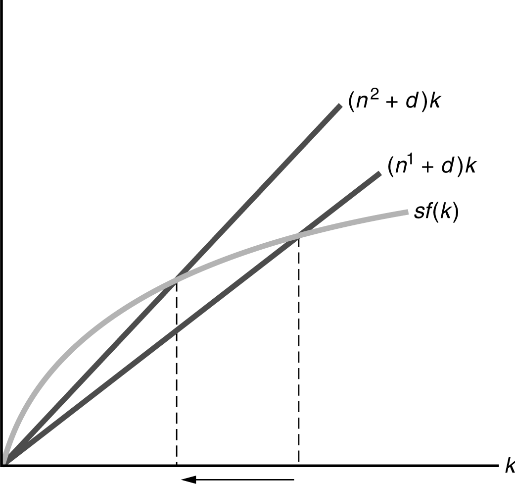
(b) Immigration raises n from n¹ to n² in Figure 6.3. The rise in n lowers steady-state k, leading to a lower steady-state consumption per worker.

Figure 6.3

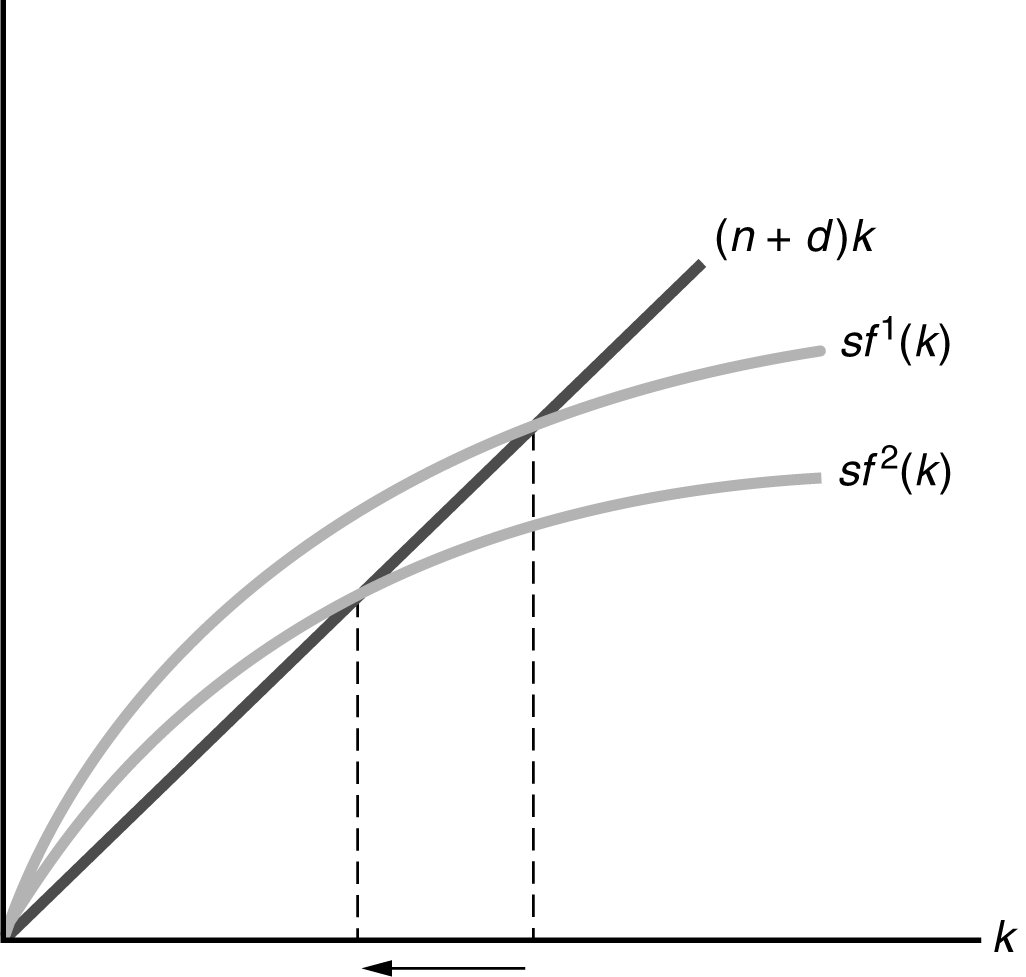
(c) A rise in energy prices reduces the productivity of capital per worker. This causes sf(k) to shift down from sf¹(k) to sf²(k) in Figure 6.4. The result is a decline in steady-state k. Steady-state consumption per worker falls for two reasons: (1) Each unit of capital has a lower productivity, and (2) steady-state k is reduced.

Figure 6.4

(d) A temporary rise in s has no long-run effect on the steady-state equilibrium.

(e) The increase in the size of the labor force does not affect the growth rate of the labor force, so there is no impact on the steady-state capital-labor ratio or on consumption per worker. This problem is similar to problem 1, but N is changing as compared to K.