1.     The position of the FE line is determined by the labor market and the production function. Labor supply and demand determine equilibrium employment. Using equilibrium employment in the production function gives the full-employment level of output. The FE line is vertical at that point. The FE line shifts to the right if there is an increase in labor supply or the capital stock or if there is a beneficial supply shock.

2.     The IS curve shows combinations of the real interest rate (r) and output (Y) that leave the goods market in equilibrium. Equilibrium in the goods market occurs when the aggregate supply of goods (Y) equals the aggregate demand for goods (C^d + I^d + G). Since desired national saving (S^d) is
Y - C^d - G, an equivalent condition is S^d = I^d. Equilibrium is achieved by the adjustment of the real interest rate to make the desired level of saving equal to the desired level of investment. For different levels of output, there are different desired saving curves, with different equilibrium interest rates. When plotted on a figure showing output and the real interest rate, this forms the IS curve, as shown in the Figure. The curve slopes downward because as output rises, the saving curve shifts along the investment curve and the real interest rate declines.

       The IS curve could shift down and to the left if: (1) expected future output falls, because this increases desired saving; (2) government purchases fall, because this increases desired saving; (3) the expected future marginal product of capital falls, because this decreases desired investment; or (4) corporate taxes increase, because this decreases desired investment.

3.     The LM curve shows the combinations of output and the real interest rate that maintain equilibrium in the asset market. Equilibrium in the asset market occurs when real money demand equals the real money supply.

        Figure 9.16 shows the derivation of the LM curve and why it slopes upward. An increase in output from Y₁ to Y₂ raises money demand, shifting the money demand curve from MD(Y₁) to MD(Y₂). With money supply fixed at MS, there must be a higher real interest rate to get equilibrium in the asset market. This gives two points of the LM curve, plotted on the right half of the figure. The result is that higher output increases the real interest rate along the LM curve, so the LM curve slopes upward.

        The LM curve would shift down and to the right if the nominal money supply or expected inflation increased or if the price level or nominal interest rate on money decreased. In addition, the curve would shift down and to the right if there were a decrease in wealth, a decrease in the risk of alternative assets relative to the risk of holding money, an increase in the liquidity of alternative assets, or an increase in the efficiency of payment technologies.

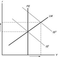
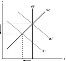
4.     General equilibrium is a situation in which all markets in an economy are simultaneously in equilibrium. This is shown in Figure below as the point at which the FE line and the IS and LM curves intersect. If the economy is not initially in general equilibrium, output and the real interest rate are determined by the intersection of the IS and LM curves. Then adjustment of the price level moves the LM curve until it intersects the FE line and IS curve.

5.     There is monetary neutrality if a change in the nominal money supply changes the price level but has no effect on real variables. Once prices adjust, money is neutral in the IS–LM model, because a change in the money supply that shifts the LM curve is matched by a proportional change in the price level that returns the real money supply back to its original level and moves the LM curve back to its original location. Classical economists believe that money is neutral in the short run, but Keynesians believe that there may be sluggish adjustment of the price level, so that changes in the money supply affect output and the real interest rate in the short run. Both classicals and Keynesians believe money is neutral in the long run.

6.     (a)  The increase in desired investment shifts the IS curve up and to the right, as shown in Figure. The price level rises, shifting the LM curve up and to the left to restore equilibrium. Since the real interest rate rises, consumption declines. In summary, there is no change in the real wage, employment, or output; there is a rise in the real interest rate, the price level, and investment; and there is a decline in consumption.

(b)  The rise in expected inflation shifts the LM curve down and to the right, as shown in Figure. The price level rises, shifting the LM curve up and to the left to restore equilibrium. Since the real interest rate is unchanged, consumption and investment are unchanged. In summary, there is no change in the real wage, employment, output, the real interest rate, consumption, or investment; and there is a rise in the price level.

(c)  The increase in labor supply is shown as a shift in the labor supply curve.
This leads to a decline in the real wage rate and an increase in employment. The rise in employment causes an increase in output, shifting the FE line to the right in Figure (b).
To restore equilibrium, the price level must decline, shifting the LM curve down and to the right. Since output increases and the real interest rate declines, consumption and investment increase.
In summary, the real wage, the real interest rate, and the price level decline; and employment, output, consumption, and investment rise.

(d)  The reduction in the demand for money gives results identical to those in part (b).

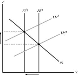
2.     The increase in the price of oil reduces the marginal product of labor, causing the labor demand curve to shift to the left from ND¹ to ND² in Figure. Since households’ expected future incomes decline, labor supply increases, shifting the labor supply curve from NS¹ to NS² (but by assumption, the shift to the left in labor demand is larger than the shift to the right in labor supply)*. At equilibrium, there is a reduced real wage and lower employment. The productivity shock results in a shift to the left of the full-employment line from FE¹ to FE² in Figure, as both employment and productivity decline. Because the shock is permanent, it reduces future output and reduces the future marginal product of capital, both of which result in a downward shift of the IS curve. The new equilibrium is located at the intersection of the new IS curve and the new FE line. If, as shown in the figure, this intersection lies above and to the left of the original LM curve, the price level will increase and shift the LM curve upward (from LM¹ to LM²) to pass through the new equilibrium point. The result is an increase in the price level, but an ambiguous effect on the real interest rate. Since output is lower, consumption is lower. Since the effect on the real interest rate is ambiguous, the effect on saving and investment are ambiguous as well, though the fall in the future marginal product of capital would tend to reduce investment.

 * It is questionable whether this second factor should be shifted now or later.

        The result is different from that of a temporary supply shock; when the shock is temporary there is no impact on future output or the marginal product of capital, so the IS curve does not shift. In that case the price level increases to shift the LM curve up and to the left from LM¹ to LM² in Figure 9.26 to restore equilibrium. In that case, the real interest rate unambiguously increases. Under a permanent shock, the IS curve shifts down and to the left, so the rise in the real interest rate is less than in the case of a temporary shock, and the real interest rate can even decline.

(a)   The decrease in expected inflation increases real money demand, shifting the LM curve up, as shown in Figure. The real interest rate rises and output declines.

(b)  The increase in desired consumption shifts the IS curve up and to the right, as shown in
Figure. This causes the real interest rate and output to rise.

(c)  The increase in government purchases shifts the IS curve up and to the right, with the same result as in part (b). (The FE line also shifts, as the increase in government expenditures reduces people’s wealth and leads them to increase labor supply, but this shift will not affect the short-run equilibrium, as the economy will be off the FE line.)

(d)  If Ricardian equivalence holds, the increase in taxes has no effect on either the IS or LM curves, so there is no change in either the real interest rate or output. If Ricardian equivalence doesn’t hold, so that the increase in taxes reduces consumption spending, the IS curve shifts down and to the left, as shown in Figure. Both the real interest rate and output decline.

(e)  An increase in the expected future marginal productivity of capital shifts the IS curve up and to the right, with the same result as in part (b).