1. If the central bank increases the money supply, then the
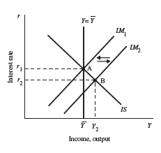
LM curve shifts downward, as shown in Figure 11–4. Income increases and the interest rate falls. Theincrease in disposable income causes consumption to rise; the fall in the interest rate causes investment to rise as well.

If government purchases increase, then the
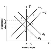
IS curve shifts to the right. This is shown in Figure 11–5. Income and the interest rate both increase. Theincrease in disposable income causes consumption to rise, while the increase in the interest rate causes investment to fall.

If the government increases taxes, then the
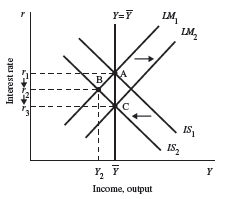
IS curve shifts to the left. This is shown in Figure 11–6. Income and the interest rate both fall. Disposable incomefalls because income is lower and taxes are higher; this causes consumption to fall. The fall in the interest rate causes investment to rise.

We can figure out how much the
IS curve shifts in response to an equal increase in government purchases and taxes by adding together the two multiplier effects. I did not expect you to do this because our focus is on the graphs and not the math, but since a few wanted to do the extra. :ΔY = [(1/(1 – MPC))]ΔG] – [(MPC/(1 – MPC))ΔT]
Because government purchases and taxes increase by the same amount, we knowthat ΔG = ΔT. Therefore, we can rewrite the above equation as:
ΔY = [(1/(1 – MPC)) – (MPC/(1 – MPC))]ΔG
ΔY = ΔG.
This expression tells us how output changes, holding the interest rate constant. It says that an equal increase in government purchases and taxes shifts the IS curve
to the right by the amount that G increases. Output increases, but by less than the amount that G and T increase; this means that disposable income Y – T falls. As a
result, consumption also falls. The interest rate rises, causing investment
2. I will let you think about #2. I wonder why I did something like this
To raise investment while keeping output constant, the government should adopt a loose monetary policy and a tight fiscal policy. (i.e. LM increases and IS decreases.) In the new equilibrium the interest rate is lower, so that investment is higher. The tight fiscal policy—reducing government purchases, for example—offsets the effect of this increase in investment on output.
The policy mix in the early 1980s did exactly the opposite. Fiscal policy was expansionary, while monetary policy was contractionary. Such a policy mix shifts the IS curve to the right and the LM curve to the left. The real interest rate rises and investment falls.
An increase in the money supply shifts the LM curve to the right in the short run. This moves the economy from point A to point B: the interest rate falls from r1 to r2, and output rises from Y to Y2. The increase in output occurs because the lower interest rate stimulates investment, which increases output.

Since the level of output is now above its long-run level, prices begin to rise. A rising price level lowers real balances, which raises the interest rate. The LM curve shifts back to the left. Prices continue to rise until the economy returns to its original position at point A. The interest rate returns to r1, and investment returns to its original level. Thus, in the long run, there is no impact on real variables from an increase in the money supply. (This is what we called monetary neutrality.)
An increase in government purchases shifts the IS curve to the right, and the economy moves from point A to point B. In the short run, output increases from Y to Y2, and the interest rate increases from r1 to r2.

The increase in the interest rate reduces investment and “crowds out” part of the expansionary effect of the increase in government purchases. Initially, the LM
curve is not affected because government spending does not enter the LM equation. After the increase, output is above its long-run equilibrium level, so prices
begin to rise. The rise in prices reduces real balances, which shifts the LM curve to the left. The interest rate rises even more than in the short run. This process
continues until the long-run level of output is again reached. At the new equilibrium, point C, interest rates have risen to r3, and the price level is permanently
higher. Note that, like monetary policy, fiscal policy cannot change the long-run level of output. Unlike monetary policy, however, it can change the composition
of output. For example, the level of investment at point C is lower than it is at point A.
An increase in taxes reduces disposable income for consumers, shifting the IS curve to the left, as shown in Figure 11–24. In the short run, output and the interest
rate decline to Y2 and r2 as the economy moves from point A to point B.

Initially, the LM curve is not affected. In the longer run, prices begin to decline because output is below its long-run equilibrium level, and the LM curve then
shifts to the right because of the increase in real money balances. Interest rates fall even further to r3 and, thus, further stimulate investment and increase
income. In the long run, the economy moves to point C. Output returns to Y, the price level and the interest rate are lower, and the decrease in consumption has
been offset by an equal increase in investment.
5. This is a funky little problem. If we did not have a virus, we might have played with this more. Given the current situation, a corona virus graph might be more important.
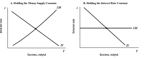
Below shows what the IS–LM model looks like for the case in which the Fed holds the money supply constant and shows what the model looks like if the Fed adjusts the money supply to hold the interest rate constant; this policy makes the effective LM curve horizontal.

If all shocks to the economy arise from exogenous changes in the demand for goods and services, this means that all shocks are to the IS curve. Suppose a shock causes
the IS curve to shift from IS1 to IS2. It is clear that output fluctuates less if the Fed follows a policy of keeping the money supply constant. Thus, if all shocks
are to the IS curve, then the Fed should follow a policy of keeping the money supply constant.

If all shocks in the economy arise from exogenous changes in the demand for money, this means that all shocks are to the LM curve. If the Fed follows a policy of adjusting the money supply to keep the interest rate constant, then the LM curve does not shift in response to these shocks—the Fed immediately adjusts the money supply to keep the money market in equilibrium. It is clear that output fluctuates less if the Fed holds the interest rate constant. If the Fed holds the interest rate constant and offsets shocks to money demand by changing the money supply, then all variability in output is eliminated. Thus, if all shocks are to the LM curve, then the Fed should adjust the money supply to hold the interest rate constant, thereby stabilizing output.
