1. (a) The predicted average test score is
![]()
(b) The predicted change in the classroom average test score is
![]()
(c) Using the formula for![]() in
Equation (4.8), we know the sample average of
the test scores across the 100 classrooms is
in
Equation (4.8), we know the sample average of
the test scores across the 100 classrooms is
![]()
(d) Use the formula for the standard error of the regression (SER) in Equation (4.19) to get the sum of squared residuals:
![]()
Use the formula for
![]() in Equation (4.16) to get the total sum of
squares:
in Equation (4.16) to get the total sum of
squares:
![]()
The sample variance is
![]()
![]() Thus, standard deviation is
Thus, standard deviation is
![]()
3. (a) The coefficient 9.6 shows the marginal effect of Age on AWE; that is, AWE is expected to increase by $9.6 for each additional year of age. 696.7 is the intercept of the regression line. It determines the overall level of the line.
(b) SER is in the same units as the dependent variable (Y, or AWE in this example). Thus SER is measures in dollars per week.
(c) R2 is unit free.
(d) (i)
![]()
(ii)
![]()
(e) No. The oldest worker in the sample is 65 years old. 99 years is far outside the range of the sample data.
(f) No. The distribution of earning is positively skewed and has kurtosis larger than the normal.
(g)
![]() so that
so that
![]() Thus the sample mean of AWE is 696.7
Thus the sample mean of AWE is 696.7
5. (a) ui represents factors other than time that influence the student’s performance on the exam including amount of time studying, aptitude for the material, and so forth. Some students will have studied more than average, other less; some students will have higher than average aptitude for the subject, others lower, and so forth.
(b) Because of random assignment ui is independent of Xi. Since ui represents deviations from average E(ui)
0. Because u and X are independent E(ui|Xi) E(ui) 0.(c) (2) is satisfied if this year’s class is typical of other classes, that is, students in this year’s class can be viewed as random draws from the population of students that enroll in the class. (3) is satisfied because 0 £ Yi £ 100 and Xi can take on only two values (90 and 120).
(d) (i)
![]()
(ii)
![]()
1. (a)
![]()
Earnings increase, on average, by 0.45 dollars per hour when workers age by 1 year.
(b) Bob’s predicted earnings
3.32 0.45 ´ 26 $11.70Alexis’s predicted earnings
3.32 0.45 ´ 30 $13.70(c) The R2 is 0.02.This mean that age explains a small fraction of the variability in earnings across individuals.
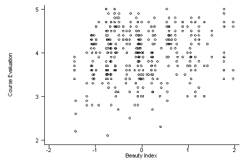
2. (a)

There appears to be a weak positive relationship between course evaluation and the beauty index.
(b)
![]()
(c) The standard deviation of Beauty is 0.789. Thus
Professor Watson’s predicted course evaluations
4.00 0.133 ´ 0 ´ 0.789 4.00Professor Stock’s predicted course evaluations
4.00 0.133 ´ 1 ´ 0.789 4.105(d) The standard deviation of course evaluations is 0.55 and the standard deviation of beauty is 0.789. A one standard deviation increase in beauty is expected to increase course evaluation by 0.133 ´ 0.789
0.105, or 1/5 of a standard deviation of course evaluations. The effect is small.(e) The regression R2 is 0.036, so that Beauty explains only 3.6% of the variance in course evaluations.